Risky Business in Stochastic Control: Exponential Utility |12 Jan. 2020|

One of the most famous problems in linear control theory is that of designing a control law which minimizes some cost being quadratic in input and state. We all know this as the Linear Quadratic Regulator (LQR) problem. There is however one problem (some would call it a blessing) with this formulation once the dynamics contain some zero-mean noise: the control law is independent of this stochasticity. This is easy in proofs, easy in practice, but does it work well? Say, your control law is rather slow, but bringing you back to in the end of time. In the noiseless case, no problem. But now say there is a substantial amount of noise, do you still want such a slow control law? The answer is most likely no since you quickly drift away. The classical LQR formulation does not differentiate between noise intensities and hence can be rightfully called naive as Bertsekas did (Bert76). Unfortunately, this name did not stuck.

Can we do better? Yes. Define the cost function

and consider the problem of finding the minimizing policy in:

Which is precisely the classical LQR problem, but now with the cost wrapped in an exponential utility function parametrized by . This problem was pioneered by most notably Peter Whittle (Wh90).

Before we consider solving this problem, let us interpret the risk parameter . For we speak of a risk-sensitive formulation while for we are risk-seeking. This becomes especially clear when you solve the problem, but a quick way to see this is to consider the approximation of near , which yields , so relates to pessimism and to optimism indeed. Here we skipped a few scaling factors, but the idea remains the same, for a derivation, consider cumulant generating functions and have a look at our problem.

As with standard LQR, we would like to obtain a stabilizing policy and to that end we will be mostly bothered with solving 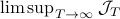. However, instead of immediately trying to solve the infinite horizon average cost Bellman equation it is easier to consider for finite first. Then, when we can prove monotonicty and upper-bound , the infinite horizon optimal policy is given by . The reason being that monotonic sequences which are uniformly bounded converge.

The main technical tool towards finding the optimal policy is the following Lemma similar to one in the Appendix of (Jac73):
Lemma
Consider a noisy linear dynamical system defined by with and let be shorthand notation for . Then, if holds we have

where .

Proof
Let and recall that the shorthand notation for is , then:

Here, the first step follows directly from being a zero-mean Gaussian. In the second step we plug in . Then, in the third step we introduce a variable with the goal of making 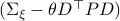the covariance matrix of a Gaussian with mean . We can make this work for

and additionally

Using this approach we can integrate the latter part to and end up with the final expression. Note that in this case the random variable needs to be Gaussian, since the second to last expression in equals by being a Gaussian probability distribution integrated over its entire domain.

What is the point of doing this? Let 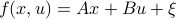and assume that 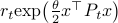represents the cost-to-go from stage and state . Then consider

Note, since we work with a sum within the exponent, we must multiply within the right-hand-side of the Bellman equation. From there it follows that , for

The key trick in simplifying your expressions is to apply the logarithm after minimizing over such that the fraction of determinants becomes a state-independent affine term in the cost. Now, using a matrix inversion lemma and the push-through rule we can remove and construct a map :

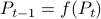such that 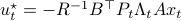. See below for the derivations, many (if not all) texts skip them, but if you have never applied the push-through rule they are not that obvious.

As was pointed out for the first time by Jacobson (Jac73), these equations are precisely the ones we see in (non-cooperative) Dynamic Game theory for isotropic and appropriately scaled .

Especially with this observation in mind there are many texts which show that 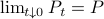is well-defined and finite, which relates to finite cost and a stabilizing control law 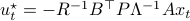. To formalize this, one needs to assume that is a minimal realization for defined by . Then you can appeal to texts like (BB95).

Numerical Experiment and Robustness Interpretation
To show what happens, we do a small -dimensional example. Here we want to solve the Risk-Sensitive ) and the Risk-neutral () infinite-horizon average cost problem for

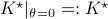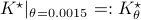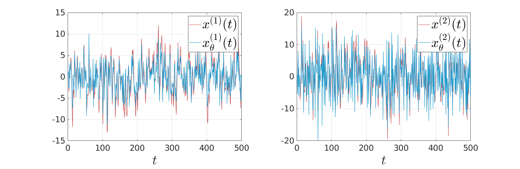
, , . There is clearly a lot of noise, especially on the second signal, which also happens to be critical for controlling the first state. This makes it interesting. We compute and . Given the noise statistics, it would be reasonable to not take the certainty equivalence control law since you control the first state (which has little noise on its line) via the second state (which has a lot of noise on its line). Let be the state under and the state under .

We see in the plot below (for some arbitrary initial condition) typical behaviour, does take the noise into account and indeed we see the induces a smaller variance.

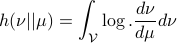
So, is more robust than in a particular way. It turns out that this can be neatly explained. To do so, we have to introduce the notion of Relative Entropy (Kullback-Leibler divergence). We will skip a few technical details (see the references for full details). Given a measure on , then for any other measure , being absolutely continuous with respect to (), define the Relative Entropy as:

Now, for any measurable function on , being bounded from below, it can be shown (see (DP96)) that

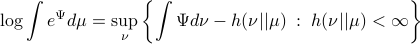
For the moment, think of as your standard finite-horizon LQR cost with product measure , then we see that an exponential utility results in the understanding that a control law which minimizes is robust against adversarial noise generated by distributions sufficiently close (measured by ) to the reference .

Here we skipped over a lot of technical details, but the intuition is beautiful, just changing the utility to the exponential function gives a wealth of deep distributional results we just touched upon in this post.

Simplification steps in
We only show to get the simpler representation for the input, the approach to obtain 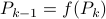is very similar.

First, using the matrix inversion lemma:

we rewrite into:

Note, we factored our since we cannot assume that is invertible. Our next tool is called the push-through rule. Given and we have

You can check that indeed . Now, to continue, plug this expression for into the input expression:

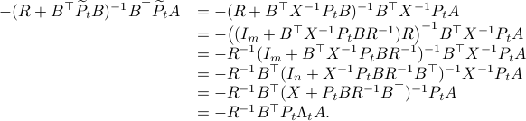
Indeed, we only used factorizations and the push-through rule to arrive here.

(Bert76) Dimitri P. Bertsekas : ‘‘Dynamic Programming and Stochastic Control’’, 1976 Academic Press.
(Jac73) D. Jacobson : ‘‘Optimal stochastic linear systems with exponential performance criteria and their relation to deterministic differential games’’, 1973 IEEE TAC.
(Wh90) Peter Whittle : ‘‘Risk-sensitive Optimal Control’’, 1990 Wiley.
(BB95) Tamer Basar and Pierre Bernhard : ‘‘-Optimal Control and Related Minimax Design Problems A Dynamic Game Approach’’ 1995 Birkhauser.
(DP96) Paolo Dai Pra, Lorenzo Meneghini and Wolfgang J. Runggaldier :‘‘Connections Between Stochastic Control and Dynamic Games’’ 1996 Math. Control Signals Systems.