Finite Calls to Stability | 31 Oct. 2019 |

Consider an unknown dynamical system $x_{k+1}=Ax_k$ parametrized by Ain mathsf{Sym}(n,mathbf{R})

. In this short note we look at a relatively simple, yet neat method to assess stability of

via finite calls to a particular oracle. Here, we will follow the notes by Roman Vershynin (RV2011).

Assume we have no knowledge of

, but we are able to obtain langle Ay, y rangle

for any desired $yin mathbf{R}^n$ . It turns out that we can use this oracle to bound rho(A)

from above.

First, recall that since

is symmetric, $|A|_2=sigma_{mathrm{max}}(A)=|lambda_{mathrm{max}}(A)|=rho(A)$ . Now, the common definition of |A|_2

is $sup_{xin mathbf{R}^nsetminus{0}}|Ax|_2/|x|_2$ . The constraint set $mathbf{R}^nsetminus{0}$ is not per se convenient from a computational point of view. Instead, we can look at a compact constraint set: $|A|_2=sup_{xin mathbf{S}^{n-1}} |Ax|_2$ , where $mathbf{S}^{n-1}$ is the sphere in $mathbf{R}^n$ . The latter formulation has an advantage, we can discretize these compact constraints sets and tame functions over the individual chunks.

To do this formally, we can use varepsilon

-nets, which are convenient in quantitative analysis on compact metric spaces (X,d)

. Let $mathcal{N}_{varepsilon}subseteq X$ be a

-net for

if $forall xin X;exists yin mathcal{N}_{varepsilon}:d(x,y)leq varepsilon$ . Hence, we measure the amount of balls to cover

For example, take $(mathbf{S}^{n-1},ell^n_2)$ as our metric space where we want to bound $|mathcal{N}_{varepsilon}|$ (the cardinality, i.e., the amount of balls). Then, to construct a minimal set of balls, consider an

-net of balls $B_{varepsilon/2}(y)$ , with $d(y_1,y_2)geq varepsilon;forall y_1,y_2in mathcal{N}_{varepsilon}$ . Now the insight is simply that $mathrm{vol}(B_{varepsilon/2})|mathcal{N}_{varepsilon}|leq mathrm{vol}(B_{1+varepsilon/2})-mathrm{vol}(B_{1-varepsilon/2})$ . Luckily, we understand the volume of

-dimensional Euclidean balls well such that we can establish

$|mathcal{N}_{varepsilon}| leq frac{mathrm{vol}(B_{1+varepsilon/2})-mathrm{vol}(B_{1-varepsilon/2})}{mathrm{vol}(B_{varepsilon/2})}= (1+2/varepsilon)^n-(1-2/varepsilon)^n.$

Next, we recite Lemma 5.4 from (RV2011). Given an varepsilon

-net for $mathbf{S}^{n-1}$ with varepsilonin[0,1)

we have

$|A|_2 = sup_{xin mathbf{S}^{n-1}}|langle Ax,xrangle | leq frac{1}{(1-2varepsilon)}sup_{xin mathcal{N}_{varepsilon}}|langle Ax,x rangle |$

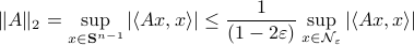
This can be shown using the Cauchy-Schwartz inequality. Now, it would be interesting to see how sharp this bound is. To that end, we do a

-dimensional example ( x=(x_1,x_2)

). Note, here we can easily find an optimal grid using polar coordinates. Let the unknown system be parametrized by

such that

. In the figures below we compute the upper-bound to |A|_2

for several nets $mathcal{N}_{varepsilon}$ . Indeed, for finer nets, we see the upper-bound approaching 0.85

. However, we see that the convergence is slow while being inversely related to the exponential growth in $|mathcal{N}_{varepsilon}|$ .

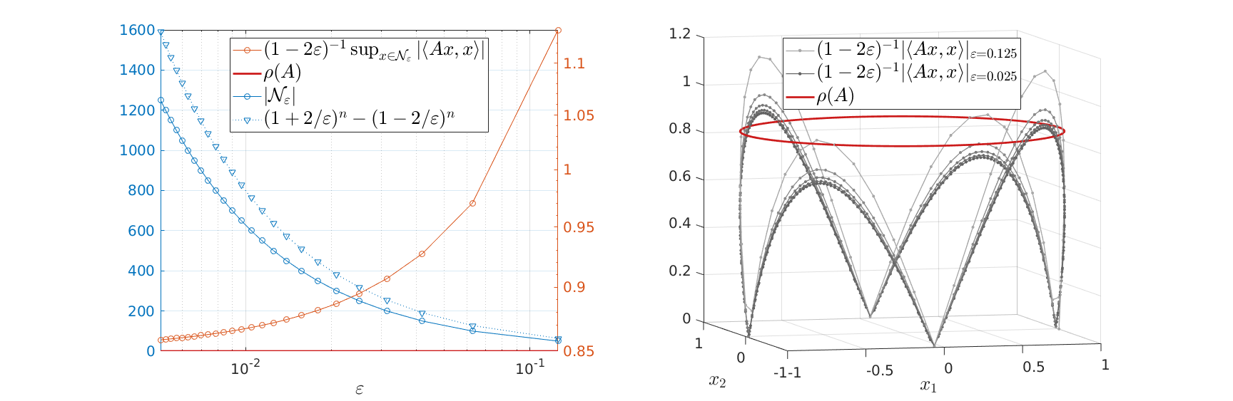Overall, we see that after about a 100 calls to our oracle we can be sure about

being exponentially stable. Here we just highlighted an example from (RV2011), at a later moment we will discuss its use in probability theory.