Counterexamples 1/N |9 January 2023|
tags: math.An

As nicely felt through the 1964 book Counterexamples in Analysis by Gelbaum and Olmsted, mathematics is not all about proving theorems, equally important is a large collection of (counter)examples to sharpen our understanding of these theorems. This attitude towards mathematics can also be found in books by Arnold, Halmos and many others.

This short post highlights a few of my favourite examples from the book by Gelbaum and Olmsted.

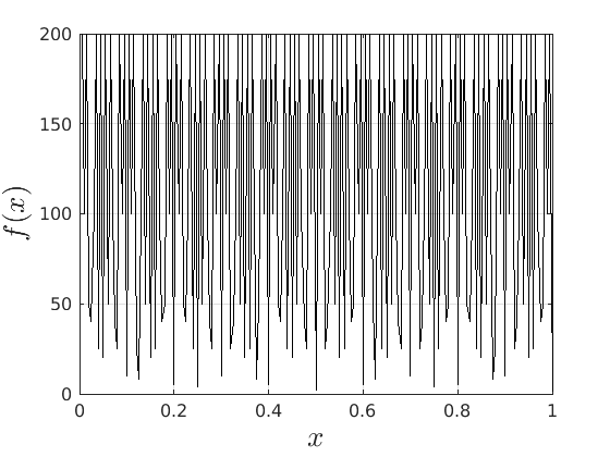
• A function that is everywhere finite and everywhere locally unbounded.

A function is locally bounded when for each point in its domain one can find a neighbourhood such that is bounded on . Now consider the function defined by

Now assume that we could locally bound on (some open neighbourhood in ), that means that is bounded on such a neighbourhood and hence, so is . However, that would imply that only contains finitely many rational numbers! We plot (approximately) below over for just points and observe precisely what one would expect.

• Two disjoint closed sets that are at a zero distance.

This example is not that surprising, but it nicely illustrates the pitfall of thinking of sets as ‘‘blobs’’ (in Dutch we would say potatoes) in the plane. Indeed, the counterexample can be interpreted as an asymptotic result. Consider 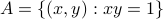, this set is closed as is continuous. Then, take 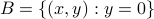, this set is again closed and clearly and are disjoint. However, since we can write , then as , we find that approaches arbitrarily closely. One can create many more examples of this form, e.g., using logarithms.

• An open and closed metric ball with the same center and radius such that the closure of the open ball is unequal to the closed ball.

This last example is again not that surprising if you are used to go beyond Euclidean spaces. Let be a metric space under the metric

Now assume that is not simply a singleton. Then, let be the open metric ball of radius centered at and similarly, let be the closed metric ball of radius centered at . Indeed, whereas . Now to construct the closure of , we must first understand the topology induced by the metric . In other words, we must understand the limit points of . Indeed, is the discrete metric and this metric induces the discrete topology on . Hence, it follows — which is perhaps the counterintuitive part, that and hence . This example also nicely shows a difference between metrics and norms. As norms satisfy 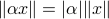(absolute homogeneity) one cannot have the discontinuous behaviour from the example above.

Further examples I particularly enjoyed are a discontinuous linear function, a function that is discontinuous in two variables, yet continuous in both variables separately and all examples related to Cantor. This post is inspired by TAing for Analysis 1 and will be continued in the near future.