Dynamical Systems on the Sphere |3 Nov. 2019|
tags: math.DS
 |
In this post we start a bit with control of systems living on compact metric spaces. This is interesting since we have to rethink what we want, |
 cannot even occur.
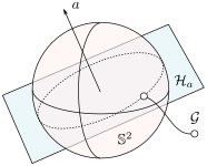
Let a great arc (circle)
cannot even occur.
Let a great arc (circle)  on
on  be parametrized by the normal of a hyperplane
  through
  ,
,  is the axis of rotation for
 To start, consider a linear dynamical systems  ,
,  , for which the solution is given by
  . We can map this solution to the sphere via
  .
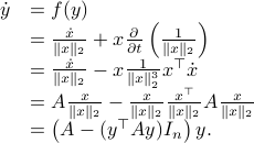
The corresponding vector field for
.
The corresponding vector field for  is given by
The beauty is the following, to find the equilibria, consider  . Of course,
  is not valid since
  . However, take any eigenvector
  of
of  , then
  is still an eigenvector, plus it lives on
  . If we plug such a scaled (from now on consider all eigenvectors to live on ) into
  we get
  , which is rather cool. The eigenvectors of are (at least) the equilibria of
  . Note, if
  , then so is
  , each eigenvector gives rise to two equilibria.
We say at least, since if
, each eigenvector gives rise to two equilibria.
We say at least, since if  is non-trivial, then for any
  , we get
  .
.
Let  , then what can be said about the stability of the equilibrium points?
Here, we must look at
, then what can be said about the stability of the equilibrium points?
Here, we must look at  , where the
  -dimensional system is locally a
  -dimensional linear system. To do this, we start by computing the standard Jacobian of
  , which is given by

As said before, we do not have a -dimensional system. To that end, we assume  with diagonalization
  (otherwise perform a Gram-Schmidt procedure) and perform a change of basis
  . Then if we are interested in the qualitative stability properties of
  (the
(the  eigenvector of ), we can simply look at the eigenvalues of the matrix resulting from removing the row and column in
  , denoted
  . This seemingly ad hoc construction heavily relies on the embedded structure.
We do two examples. In both figures are the initial conditions indicated with a dot while the equilibrium points are stars.
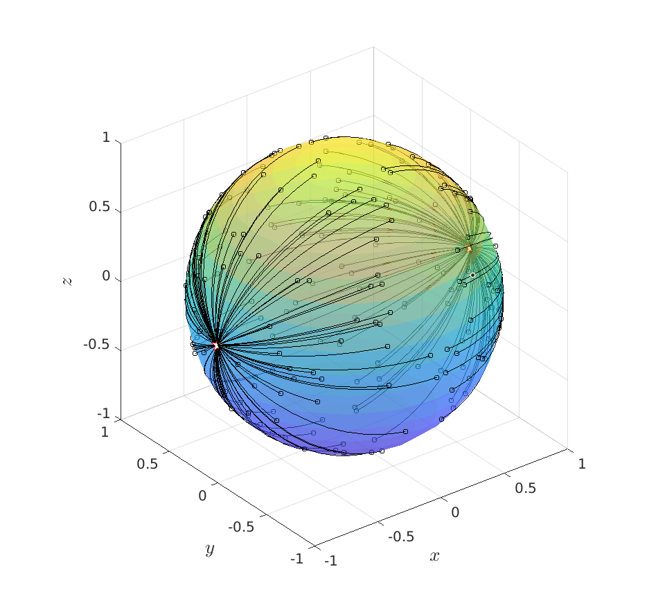 |
First, let ![A_1 = left[ begin{array}{lll} 1 & 0 & 0 0 & -1 & 0 0 & 0 & -1 end{array}right]](eqs/4948366788842116208-130.png)
Clearly, for |
 we have
  and let
  be
be  . Then using the procedure from before, we find that
  is stable (attracting), while
  are locally unstable in one direction while
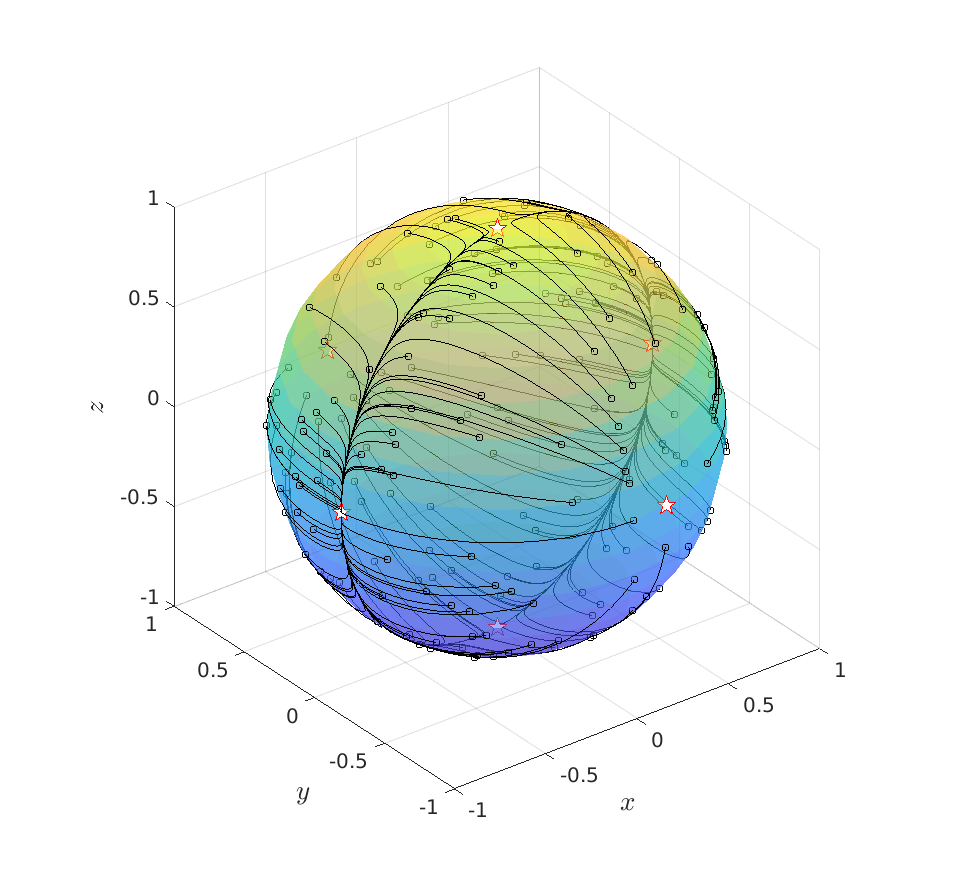 |
Secondly, we consider ![A_2 = left[ begin{array}{lll} 1 & 2 & 0 2 & -10 & 0 0 & 0 & 0.1 end{array}right]](eqs/5655966812910521664-130.png)
To assess stability, we compute ![Df'|_{T_{v_1}mathbf{S}^{2}} = left[ begin{array}{ll} 11.7 & 0 0 & 10.4 end{array}right],quad Df'|_{T_{v_2}mathbf{S}^{2}} = left[ begin{array}{ll} -11.7 & 0 0 & -1.2 end{array}right],quad Df'|_{T_{v_3}mathbf{S}^{2}} = left[ begin{array}{ll} -10.4 & 0 0 & 1.2 end{array}right].](eqs/3105021875749429669-130.png)
Recall that tangent space basis is in line with the eigenvectors plus that the qualitative behaviour around |
 for
for  and
and  ,
,  ,
,  ,
,  :
:  equals that around
  . This explains the attracting great arc parametrized by
  . Note, although the arc is attracting,
  does not vanish on the complete arc, we are locally unstable along
  and therefore converge to
  .
. Now, a valid question is, why do stable equilibrium points (for on  ) become unstable on the sphere?
For our example, we see that the full (minus
) become unstable on the sphere?
For our example, we see that the full (minus  ) line: all
  s.t.
s.t.  collapses to just two points:
  . Not just any two points, but two points surrounded by instability, hence the positive definite Jacobian. In a similar fashion it follows that the unstable asymptotes
  now relate to (finite!) attracting equilibria
  . The fact that
  is attracting from all directions while
  relates to a saddle follows from the corresponding eigenvalues,
  .
From the figure you can take away that
.
From the figure you can take away that  is the attracting plane, resulting in
  being an attracting great arc (since
  ).
).
We observe that by construction it seems impossible to have 1 stable pole since the equilibrium points come in pairs. You might say, sure, but these vector fields where created by using linear systems. Perhaps there is some wild differential equation which does the trick? The answer is yes, we can however not remove the equilibrium points completely, we cannot comb a hairy ball.