Posts (11) containing the 'math.DS’ (Dynamical Systems) tag:
On Critical Transitions in Nature and Society |29 January 2023|
tags: math.DS
The aim of this post is to highlight the 2009 book Critical Transitions in Nature and Society by Prof. Scheffer, which is perhaps more timely than ever and I strongly recommend this book to essentially anyone.
Far too often we (maybe not you) assume that systems are simply reversible, e.g. based on overly simplified models (think of a model corresponding to a flow). The crux of this book is that for many ecosystems such a reversal might be very hard or even practically impossible. Evidently, this observation has many serious ramifications with respect to understanding and tackling climate change.
Mathematically, this can be understood via bifurcation theory, in particular, via folds and cusps, introducing a form of hysteresis. The hysteresis is important here, as this means that simply restoring some parameters of an ecosystem does not directly imply that the state of the ecosystem will return to what these parameters were previously corresponding to.
The book makes a good point that catastrophe- and chaos theory (old friends of bifurcation theory) themselves went through a critical transition, that is, populair media (and some authors) blew-up those theories. To that end, see the following link for a crystal clear introduction to catastrophe theory by Zeeman (including some controversy), as well as this talk by Ralph Abraham on the history (locally) of chaos theory. One might argue that some populair fields these days are also trapped in a similar situation.
Scheffer stays away from drawing overly strong conclusions and throughout the book one can find many discussions on how and if to relate these models to reality. Overall, Scheffer promotes system theoretic thinking. For example, at first sight we might be inclined to link big (stochastic) events, e.g. a meteor hitting the earth, as the cause of some disruptive event, while actually something else might been slowly degrading, e.g. some basin of attraction shrunk, and this stochastic event was just the final push. This makes the book very timely, climate change is slowly changing ecosystems around us, we are just waiting for a detrimental push. To give another example, in Chapter 5 we find an interesting discussion on the relation between biodiversity and stability. Scheffer highlights two points: (i) robustness (there is plently back-up) and (ii) complementation (if many can perform a task, some of them will be very good at it). Overall, the discussions on ‘‘why we have so many animals’’ are very interesting.
One of the main concepts in the book is that of resilience, which is (re)-defined several times (as part of the storyline in the book), in particular, one page 103 we find it being defined as ‘‘the capacity of a system to absorb disturbance and reorganize while undergoing change so as to still retain essentially the same function, structure, identity, and feedbacks.’’ Qualitatively, this is precisely a combination of having an attractor of some system being structurally stable. However, the goal here is to quantify this structural stability to some extent. Indeed, one enters bifurcation theory, or if you like, topological dynamical systems theory.
Throughout, Scheffer provides incredibly many examples of great inspiration to anyone in dynamical system and control theory, e.g. the basin of attraction, multistability and time-separations are recurring themes. My favourite simple example (of positive feedback) being the ice-Albedo feedback, (too) simply put, less ice means less reflection of light and hence more heat absorption, resulting in even less ice (as such, the positive feedback). More details can be found in Chapter 8. Another detailed series of examples is contained in Chapter 7 on shallow lakes. This chapter explains through a qualitative lens why restoring lakes is inherently difficult. Again, (too) simply put, as with ice, if plants disappear in lakes, turbidity is promoted, making it more difficult for plants to return (they need sunlight and thus prefer clear water). For this lake model, one can find some equations in Appendix 12, which is essentially a Lotka-Volterra model. As such, some readers might be unsatisfied when it comes to the mathematical content*. Moreover, at times Scheffer himself describes bifurcations as exotic dynamical systems jargon and throughout the book one might get the feeling that the dynamical systems community has no clue how to handle time-varying models. Luckily, the latter is not completely true. Perhaps the crux here is that we can use more cross-contamination between scientific communities. Especially recognizing these bifurcations (critical transitions), not just in models, but in reality is still a big and pressing open problem.
*A fantastic and easy-going short book on catastrophe theory is written, of course, by Arnold.
The aim of this book was to have a widely accesible mathematical reference. The introduction to this book reads as: ‘‘This booklet explains what catastrophe theory is about and why it arouses such controversy. It also contains non-controversial results from the mathematical theories of singularities and bifurcation.’’
whereas Arnold ends with: ‘‘A qualitative peculiarity of Thom's papers on catastrophe theory is their original style: as one who presenses the direction of future investigations, Thom not only does not have proofs available, but does not even dispose of the precise formulations of his results. Zeeman, an ardent admirer of this style, observes that the meaning of Thom's words becomes clear only after inserting 99 lines of your own between every two of Thom's.’’
On ‘‘the art of the state’’ |29 December 2022|
tags: math.DS
In the last issue of the IEEE Control Systems Magazine, Prof. Sepulchre wrote an exhilarating short piece on the art of the state, or as he (also) puts it ‘‘the definite victory of computation over modeling in science and engineering’’. As someone with virtually no track record, I am happy to also shed my light on the matter.
We owe dynamical systems theory as we know it today largely to Henri Poincaré (1854-1912), whom started this in part being motivated by describing the solar system. Better yet, the goal was to eventually understand its stability. However, we can be a bit more precise regarding what was driving all this work. In the introduction of Les méthodes nouvelles de la mécanique céleste (EN: The new methods of celestial mechanics) - Vol I by Poincaré, published in 1892 (HP92), we find (loosely translated): ‘‘The ultimate goal of Celestial Mechanics is to resolve this great question of whether Newton's law alone explains all astronomical phenomena; the only way to achieve this is to make observations as precise as possible and then compare them with the results of the calculation.’’ and then after a few words on divergent series: ‘‘these developments should attract the attention of geometers, first for the reasons I have just explained and also for the following: the goal of Celestial Mechanics is not reached when one has calculated more or less approximate ephemerides without being able to realize the degree of approximation obtained. If we notice, in fact, a discrepancy between these ephemerides and the observations, we must be able to recognize if Newton's law is at fault or if everything can be explained by the imperfection of the theory.’’ It is perhaps interesting to note that his 1879 thesis entitled: Sur les propriétés des fonctions définies par les équations aux différences partielles (EN: On the properties of functions defined by partial difference equations) was said to lack examples (p.109 FV12).
In the 3 Volumes and well over a 1000 pages of the new celestial mechanics Poincaré develops a host of tools towards the goal sketched above. Indeed, this line of work contributed to the popularizing of the infamous equation
or as used in control theory:  , for
, for  some ‘‘update’’ operator. However, I would like to argue that the main issue with Equation
  is not that it is frequently used, but how it is used, moving from the qualitative to the quantitative.
Unfortunately we cannot ask him, but I believe Poincaré would wholeheartedly agree with Sepulchre. Inspired by the beautiful book by Prof. Verhulst (FV12) I will try to briefly illustrate this claim. As put by Verhulst (p.80 FV12): ‘‘In his writings, Poincaré was interested primarily in obtaining insight into physical reality and mathematical reality — two different things.’’ In fact, the relation between analysis and physics was also the subject of Poincaré’s plenary lecture at the first International Congress of Mathematicians, in Zurich (1897). (p.91 FV12).
In what follows we will have a closer look at La Valeur de la Science (EN: The value of science) by Poincaré, published in 1905 (HP05). This is one of his more philosophical works. We already saw how Poincaré was largely motivated by a better understanding of physics. We can further illustrate how he — being one of the founders of many abstract mathematical fields — thought of physics. To that end, consider the following two quotes:
’’when physicists ask of us the solution of a problem, it is not a duty-service they impose upon us, it is on the contrary we who owe them thanks.’’ (p.82 HP05)
‘‘Fourier's series is a precious instrument of which analysis makes continual use, it is by this means that it has been able to represent discontinuous functions; Fourier invented it to solve a problem of physics relative to the propagation of heat. If this problem had not come up naturally, we should never have dared to give discontinuity its rights; we should still long have regarded continuous functions as the only true functions.’’ (p.81 HP05)
What is more, this monograph contains a variety of discussions of the form: ’’If we assume A, B and C, what does this imply?’’ Both mathematically and physically. For instance, after a discussion on Carnot's Theorem (principle) — or if you like the ramifications of a global flow — Poincaré writes the following:
‘‘On this account, if a physical phenomenon is possible, the inverse phenomenon should be equally so, and one should be able to reascend the course of time. Now, it is not so in nature, …’’ (p.96 HP05)
However, Poincaré continues and argues that although notions like friction seem to lead to an irreversible process this is only so because we look at the process through the wrong lens.
‘‘For those who take this point of view, Carnot's principle is only an imperfect principle, a sort of concession to the infirmity of our senses; it is because our eyes are too gross that we do not distinguish the elements of the blend; it is because our hands are too gross that we can not force them to separate; the imaginary demon of Maxwell, who is able to sort the molecules one by one, could well constrain the world to return backward.’’ (p.97 HP05)
Indeed, the section is concluded by stating that perhaps we should look through the lens of statistical mechanics. All to say that if the physical reality is ought the be described, this must be on the basis of solid principles. Let me highlight another principle: conservation of energy. Poincaré writes the following:
‘‘I do not say: Science is useful, because it teaches us to construct machines. I say: Machines are useful, because in working for us, they will some day leave us more time to make science.’’ (p.88 HP05)
‘‘Well, in regard to the universe, the principle of the conservation of energy is able to render us the same service. The universe is also a machine, much more complicated than all those of industry, of which almost all the parts are profoundly hidden from us; but in observing the motion of those that we can see, we are able, by the aid of this principle, to draw conclusions which remain true whatever may be the details of the invisible mechanism which animates them.’’ (p.94 HP05)
Then, a few pages later, his brief story on radium starts as follows:
‘‘At least, the principle of the conservation of energy yet remained to us, and this seemed more solid. Shall I recall to you how it was in its turn thrown into discredit?’’ (p.104 HP05)
Poincaré his viewpoint is to some extent nicely captured by the following piece in the book by Verhulst:
‘‘Consider a mature part of physics, classical mechanics (Poincaré 02). It is of interest that there is a difference in style between British and continental physicists. The former consider mechanics an experimental science, while the physicists in continental Europe formulate classical mechanics as a deductive science based on a priori hypotheses. Poincaré agreed with the English viewpoint, and observed that in the continental books on mechanics, it is never made clear which notions are provided by experience, which by mathematical reasoning, which by conventions and hypotheses.’’ (p.89 FV12)
In fact, for both mathematics and physics Poincaré spoke of conventions, to be understood as a convenience in physics. Overall, we see that Poincaré his attitude to applying mathematical tools to practical problems is significantly more critical than what we see nowadays in some communities. For instance:
‘‘Should we simply deduce all the consequences, and regard them as intangible realities? Far from it; what they should teach us above all is what can and what should be changed.’’ (p.79 HP05)
A clear example of this viewpoint appears in his 1909 lecture series at Göttingen on relativity:
‘‘Let us return to the old mechanics that admitted the principle of relativity. Instead of being founded on experiment, its laws were derived from this fundamental principle. These considerations were satisfactory for purely mechanical phenomena, but the old mechanics didn’t work for important parts of physics, for instance optics.’’ (p.209 FV12)
Now it is tempting to believe that Poincaré would have liked to get rid of ‘‘the old’’, but this is far from the truth.
‘‘We should not have to regret having believed in the principles, and even, since velocities too great for the old formulas would always be only exceptional, the surest way in practise would be still to act as if we continued to believe in them. They are so useful, it would be necessary to keep a place for them. To determine to exclude them altogether would be to deprive oneself of a precious weapon.’’ (p.111 HP05)
The previous was about the ‘‘old’’ and ‘‘new’’ mechanics and how differences in mathematical and physical realities might emerge. Most and for all, the purpose of the above is to show that one of the main figures in abstract dynamical system theory — someone that partially found the field motivated by a computational question — greatly cared about correct modelling.
This is one part of the story. The second part entails the recollection that Poincaré his work was largely qualitative. Precisely this qualitative viewpoint allows for imperfections in the modelling process. However, this also means conclusions can only be qualitative. To provide two examples; based on the Hartman-Grobman theorem and the genericity of hyperbolic equilibrium points it is perfectly reasonable to study linear dynamical systems, however, only to understand local qualitative behaviour of the underlying nonlinear dynamical system. The aim to draw quantitative conclusions is often futile and simply not the purpose of the tools employed. Perhaps more interesting and closer to Poincaré, the Lorenz system, being a simplified mathematical model for atmospheric convection, is well-known for being chaotic. Now, weather-forecasters do use this model, not to predict the weather, but to elucidate why their job is hard!
Summarizing, I believe the editorial note by Prof. Sepulchre is very timely as some have forgotten that the initial dynamical systems work by Poincaré and others was to get a better understanding, to adress questions, to learn from, not to end with. Equation (1) is not magical, but a tool to build the bridge, a tool to see if and where the bridge can be built.
A corollary |6 June 2022|
tags: math.DS
The lack of mathematically oriented people in the government is an often observed phenomenon |1|. In this short note we clarify that this is a corollary to ‘‘An application of Poincare's recurrence theorem to adademic adminstration’’, by Kenneth R. Meyer. In particular, since the governmental system is qualitatively the same as that of academic administration, it is also conservative. However - due to well-known results also pioneered by Poincare - this implies the following.
Corollary: The government is non-exact.
Solving Linear Programs via Isospectral flows |05 September 2021|
tags: math.OC, math.DS, math.DG
In this post we will look at one of the many remarkable findings by Roger W. Brockett. Consider a Linear Program (LP)

parametrized by the compact set  and a suitable triple
  .
As a solution to can always be found to be a vertex of
.
As a solution to can always be found to be a vertex of  , a smooth method to solve seems somewhat awkward.
We will see that one can construct a so-called isospectral flow that does the job.
Here we will follow Dynamical systems that sort lists, diagonalize matrices and solve linear programming problems, by Roger. W. Brockett (CDC 1988) and the book Optimization and Dynamical Systems edited by Uwe Helmke and John B. Moore (Springer 2ed. 1996).
Let have
, a smooth method to solve seems somewhat awkward.
We will see that one can construct a so-called isospectral flow that does the job.
Here we will follow Dynamical systems that sort lists, diagonalize matrices and solve linear programming problems, by Roger. W. Brockett (CDC 1988) and the book Optimization and Dynamical Systems edited by Uwe Helmke and John B. Moore (Springer 2ed. 1996).
Let have  vertices, then one can always find a map
  , mapping the simplex
  onto .
Indeed, with some abuse of notation, let
onto .
Indeed, with some abuse of notation, let  be a matrix defined as
  , for
, for  , the vertices of .
Before we continue, we need to establish some differential geometric results. Given the Special Orthogonal group  , the tangent space is given by
  . Note, this is the explicit formulation, which is indeed equivalent to shifting the corresponding Lie Algebra.
The easiest way to compute this is to look at the kernel of the map defining the underlying manifold.
. Note, this is the explicit formulation, which is indeed equivalent to shifting the corresponding Lie Algebra.
The easiest way to compute this is to look at the kernel of the map defining the underlying manifold.
Now, following Brockett, consider the function  defined by
  for some
  . This approach is not needed for the full construction, but it allows for more intuition and more computations.
To construct the corresponding gradient flow, recall that the (Riemannian) gradient at
. This approach is not needed for the full construction, but it allows for more intuition and more computations.
To construct the corresponding gradient flow, recall that the (Riemannian) gradient at  is defined via
 ![df(Theta)[V]=langle mathrm{grad},f(Theta), Vrangle_{Theta}](eqs/666734593389601294-130.png) for all
for all  . Using the explicit tangent space representation, we know that
  with
with  .
Then, see that by using
.
Then, see that by using

we obtain the gradient via
![df(Theta)[V]=lim_{tdownarrow 0}frac{f(Theta+tV)-f(Theta)}{t} = langle QTheta N, Theta Omega rangle - langle Theta N Theta^{mathsf{T}} Q Theta, Theta Omega rangle.](eqs/2651725126600601485-130.png)
This means that (the minus is missing in the paper) the (a) gradient flow becomes

Consider the standard commutator bracket ![[A,B]=AB-BA](eqs/2726051070798907854-130.png) and see that for
and see that for  one obtains from the equation above (typo in the paper)
![dot{H}(t) = [H(t),[H(t),N]],quad H(0)=Theta^{mathsf{T}}QThetaquad (2).](eqs/8308117426617579905-130.png)
Hence,  can be seen as a reparametrization of a gradient flow.
It turns out that has a variety of remarkable properties. First of all, see that
can be seen as a reparametrization of a gradient flow.
It turns out that has a variety of remarkable properties. First of all, see that  preserves the eigenvalues of
  .
Also, observe the relation between extremizing
.
Also, observe the relation between extremizing  and the function
  defined via
  . The idea to handle LPs is now that the limiting will relate to putting weight one the correct vertex to get the optimizer,
  gives you this weight as it will contain the corresponding largest costs.
In fact, the matrix  can be seen as an element of the set
  .
This set is in fact a
.
This set is in fact a  -smooth compact manifold as it can be written as the orbit space corresponding to the group action
  ,
,
 , one can check that this map satisfies the group properties. Hence, to extremize over
  , it appears to be appealing to look at Riemannian optimization tools indeed. When doing so, it is convenient to understand the tangent space of
  . Consider the map defining the manifold
  ,
,  . Then by the construction of
  , see that
 ![dh(Theta)[V]=0](eqs/8898228761859333701-130.png) yields the relation
yields the relation ![[H,Omega]=0](eqs/197549272010137556-130.png) for any
for any  .
.
For the moment, let  such that
  and
and  .
First we consider the convergence of .
Let have only distinct eigenvalues, then
.
First we consider the convergence of .
Let have only distinct eigenvalues, then  exists and is diagonal.
Using the objective from before, consider
exists and is diagonal.
Using the objective from before, consider  and see that by using the skew-symmetry one recovers the following
![begin{array}{lll} frac{d}{dt}mathrm{Tr}(H(t)N) &=& mathrm{Tr}(N [H,[H,N]]) &=& -mathrm{Tr}((HN-NH)^2) &=& |HN-NH|_F^2. end{array}](eqs/6018522323896655448-130.png)
This means the cost monotonically increases, but by compactness converges to some point  . By construction, this point must satisfy
 ![[H_{infty},N]=0](eqs/5408610946697229240-130.png) . As has distinct eigenvalues, this can only be true if itself is diagonal (due to the distinct eigenvalues).
. As has distinct eigenvalues, this can only be true if itself is diagonal (due to the distinct eigenvalues).
More can be said about , let  be the eigenvalues of
  , that is, they correspond to the eigenvalues of as defined above.
Then as preserves the eigenvalues of (), we must have
, that is, they correspond to the eigenvalues of as defined above.
Then as preserves the eigenvalues of (), we must have  , for
, for  a permutation matrix.
This is also tells us there is just a finite number of equilibrium points (finite number of permutations). We will write this sometimes as
a permutation matrix.
This is also tells us there is just a finite number of equilibrium points (finite number of permutations). We will write this sometimes as  .
.
Now as is one of those points, when does converge to ? To start this investigation, we look at the linearization of , which at an equilibrium point becomes

for  . As we work with matrix-valued vector fields, this might seems like a duanting computation. However, at equilibrium points one does not need a connection and can again use the directional derivative approach, in combination with the construction of
  , to figure out the linearization. The beauty is that from there one can see that is the only asymptotically stable equilibrium point of . Differently put, almost all initial conditions
  will converge to with the rate captured by spectral gaps in and . If does not have distinct eigenvalues and we do not impose any eigenvalue ordering on , one sees that an asymptotically stable equilibrium point must have the same eigenvalue ordering as . This is the sorting property of the isospectral flow and this is of use for the next and final statement.
Theorem:
Consider the LP with  for all
 ![i,jin [k]](eqs/5752860898065984697-130.png) , then, there exist diagonal matrices and
such that converges for almost any to
, then, there exist diagonal matrices and
such that converges for almost any to  with the optimizer of being
  .
.
Proof:
Global convergence is prohibited by the topology of .
Let  and let
  . Then, the isospectral flow will converge from almost everywhere to
  (only
(only  ), such that
  .
.
Please consider the references for more on the fascinating structure of .
Topological Considersations in Stability Analysis |17 November 2020|
tags: math.DS
In this post we discuss very classical, yet, highly underappreciated topological results.
We will look at dynamical control systems of the form

where  is some finite-dimensional embedded manifold.
As it turns out, topological properties of encode a great deal of fundamental control possibilities, most notably, if a continuous globally asymptotically stabilizing control law exists or not (usually, one can only show the negative). In this post we will work towards two things, first, we show that a technically interesting nonlinear setting is that of a dynamical system evolving on a compact manifold, where we will discuss that the desirable continuous feedback law can never exist, yet, the boundedness implied by the compactness does allow for some computations. Secondly, if one is determined to work on systems for which a continuous globally asymptotically stable feedback law exists, then a wide variety of existential sufficient conditions can be found, yet, the setting is effectively Euclidean, which is the most basic nonlinear setting.
To start the discussion, we need one important topological notion.
Definition [Contractability].
Given a topological manifold  . If the map
  is null-homotopic, then, is contractible.
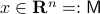
To say that a space is contractible when it has no holes (genus  ) is wrong, take for example the sphere. The converse is true, any finite-dimensional space with a hole cannot be contractible. See Figure 1 below.
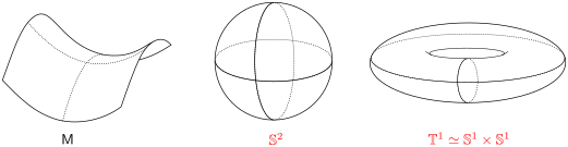 |
Figure 1:
The manifold |
Topological Obstructions to Global Asymptotic Stability
In this section we highlight a few (not all) of the most elegant topological results in stability theory. We focus on results without appealing to the given or partially known vector field .
This line of work finds its roots in work by Bhatia, Szegö, Wilson, Sontag and many others.
Theorem [The domain of attraction is contractible, Theorem 21]
Let the flow  be continuous and let
  be an asymptotically stable equilibrium point. Then, the domain of attraction
  is contractible.
This theorem by Sontag states that the underlying topology of a dynamical system, better yet, the space on which the dynamical system evolves, dictates what is possible. Recall that linear manifolds are simply hyperplanes, which are contractible and hence, as we all know, global asymptotic stability is possible for linear systems. However, if is not contractible, there does not exist a globally asymptotically stabilizable continuous-time system on , take for example any sphere.
The next example shows that one should not underestimate ‘‘linear systems’’ either.
Example [Dynamical Systems on  ]
Recall that
]
Recall that  is a smooth
  -dimensional manifold (Lie group).
Then, consider for some
-dimensional manifold (Lie group).
Then, consider for some  ,
,  the (right-invariant) system

Indeed, the solution to (1) is given by  . Since this group consists out of two disjoint components there does not exist a matrix
  , or continuous nonlinear map for that matter, which can make a vector field akin to (1) globally asymptotically stable. This should be contrasted with the closely related ODE
  ,
,  . Even for the path connected component
  , The theorem by Sontag obstructs the existence of a continuous global asymptotically stable vector field. This because the group is not simply connected for (This follows most easily from establishing the homotopy equivalence between
  and
and  via (matrix) Polar Decomposition), hence the fundamental group is non-trivial and contractibility is out of the picture. See that if one would pick to be stable (Hurwitz), then for
  we have
 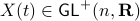 , however
 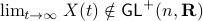 .
.
Following up on Sontag, Bhat and Bernstein revolutionized the field by figuring out some very important ramifications (which are easy to apply). The key observation is the next lemma (that follows from intersection theory arguments, even for non-orientable manifolds).
Lemma [Proposition 1] Compact, boundaryless, manifolds are never contractible.
Clearly, we have to ignore -dimensional manifolds here. Important examples of this lemma are the  -sphere
  and the rotation group
  as they make a frequent appearance in mechanical control systems, like a robotic arm.
Note that the boundaryless assumption is especially critical here.
as they make a frequent appearance in mechanical control systems, like a robotic arm.
Note that the boundaryless assumption is especially critical here.
Now the main generalization by Bhat and Bernstein with respect to the work of Sontag is to use a (vector) bundle construction of .
Loosely speaking, given a base  and total manifold , is a vector bundle when for the surjective map
  and each
  we have that the fiber
  is a finite-dimensional vector space (see the great book by Abraham, Marsden and Ratiu Section 3.4 and/or the figure below).
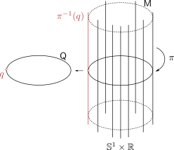 |
Figure 2:
A prototypical vector bundle, in this case the cylinder |
Intuitively, vector bundles can be thought of as manifolds with vector spaces attached at each point, think of a cylinder living in  , where the base manifold is
  and each fiber is a line through
  extending in the third direction, as exactly what the figure shows. Note, however, this triviality only needs to hold locally.
A concrete example is a rigid body with 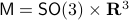 , for which a large amount of papers claim to have designed continuous globally asymptotically stable controllers. The fact that this was so enormously overlooked makes this topological result not only elegant from a mathematical point of view, but it also shows its practical value.
The motivation of this post is precisely to convey this message, topological insights can be very fruitful.
, for which a large amount of papers claim to have designed continuous globally asymptotically stable controllers. The fact that this was so enormously overlooked makes this topological result not only elegant from a mathematical point of view, but it also shows its practical value.
The motivation of this post is precisely to convey this message, topological insights can be very fruitful.
Now we can state their main result
Theorem [Theorem 1]
Let  be a compact, boundaryless, manifold, being the base of the vector bundle
  with
with  , then, there is no continuous vector field on with a global asymptotically stable equilibrium point.
Indeed, compactness of can also be relaxed to not being contractible as we saw in the example above, however, compactness is in most settings more tangible to work with.
Example [The Grassmannian manifold]
The Grassmannian manifold, denoted by  , is the set of all -dimensional subspaces
  . One can identify with the Stiefel manifold
  , the manifold of all orthogonal -frames, in the bundle sense of before, that is
 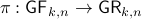 such that the fiber
  represent all -frames generating the subspace
  . In its turn, can be indentified with the compact Lie group
  (via a quotient), such that indeed is compact.
This manifold shows up in several optimization problems and from our continuous-time point of view we see that one can never find, for example, a globally converging gradient-flow like algorithm.
(via a quotient), such that indeed is compact.
This manifold shows up in several optimization problems and from our continuous-time point of view we see that one can never find, for example, a globally converging gradient-flow like algorithm.
Example [Tangent Bundles]
By means of a Lagrangian viewpoint, a lot of mechanical systems are of a second-order nature, this means they are defined on the tangent bundle of some , that is,  . However, then, if the configuration manifold is compact, we can again appeal to the Theorem by Bhat and Bernstein. For example, Figure 2 can relate to the manifold over which the pair
  is defined.
Global Isomorphisms
One might wonder, given a vector field over a manifold , since we need contractibility of for to have a global asymptotically stable equilibrium points, how interesting are these manifolds? As it turns out, for  , which some might call the high-dimensional topological regime, contractible manifolds have a particular structure.
A topological space being simply connected is equivalent to the corresponding fundamental group being trivial. However, to highlight the work by Stallings, we need a slightly less well-known notion.
Definition [Simply connected at infinity]
The topological space is simply connected at infinity, when for any compact subset  there exists a
  where
where  such that
  is simply connected.
This definition is rather complicated to parse, however, we can give a more tangible description. Let be a non-compact topological space, then, is said to have one end when for any compact  there is a where such that is connected. So,
  , as expected, fails to have one end, while
  does have one end.
Now, Proposition 2.1 shows that if and
does have one end.
Now, Proposition 2.1 shows that if and  are simply connected and both have one end, then
  is simply connected at infinity. This statement somewhat clarifies why dimension
  and above are somehow easier to parse in the context of topology. A similar statement can be made about the cylindrical space
  .
.
Lemma [Product representation Proposition 2.4]
Let and be manifolds of dimension greater or equal than  . If
. If  is contractible and
  , then, is simply connected at infinity.
Now, most results are usually stated in the context of a piecewise linear (PL) topology. By appealing to celebrated results on triangulization (by Whitehead) we can state the following.
Theorem [Global diffeomorphism Theorem 5.1]
Let be a contractible  ,
,  , -dimensional manifold which is simply connected at infinity. If , then, is diffeomorphic to
  .
.
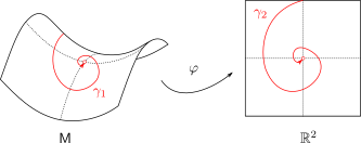 |
Figure 3:
The manifold |
 is usually much easier than dealing with
  directly.
 You might say that this is all obvious, as in Figure 3, we can always do it, also for lower-dimensions. However, there is famous counterexample by Whitehead, which provided lots of motivation for the community:
‘‘There is an open,  -dimensional manifold which is contractible, but not homeomorphic to .’’
In fact, this example was part of the now notorious program to solve the Poincaré conjecture. All in all, this shows that contractible manifolds are not that interesting from a nonlinear dynamical systems point of view, compact manifolds is a class of manifolds providing for more of a challenge.
Remark on the Stabilization of Sets
So far, the discussion has been on the stabilization of (equilibrium) points, now what if we want to stabilize a curve or any other desirable set, that is, a non-trivial set  . It seems like the shape of these objects, with respect to the underlying topology of , must indicate if this is possible again? Let
  denote an open neighbourhood of some
  . In what follows, the emphasis is on
  and having the same topology. We will be brief and follow Moulay and Bhat.
Lemma [Theorem 5]
Consider a closed-loop dynamical system given rise to a continuous flow. Suppose that the compact set  is asymptotically stable with domain of attraction
  . Then, is a weak deformation retract of
  .
.
In rather loose terms, being a weak deformation retract of means that one can continuously ‘‘retract’’ points from and morph them into the set . So, this works for and  , due to being punctured. See p.200 for more information on retracts. In Figure 4 below we show that since this lemma is mostly concerned with the local topology, the global topology is less important. For , the set is not a deformation retract of the set
  such that can never be a region of attraction, this should be contrasted with the setting on the Torus
  .
.
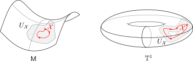 |
Figure 4:
The topological relation between |
The beauty of all of this is that even if you are not so sure about the exact dynamical system at hand, the underlying topology can already provide for some answers. In particular, to determine, what can, or cannot be done.
This post came about during a highly recommended course at EPFL.
Optimal coordinates |24 May 2020|
tags: math.LA, math.OC, math.DS
There was a bit of radio silence, but as indicated here, some interesting stuff is on its way.
In this post we highlight this 1976 paper by Mullis and Roberts on ’Synthesis of Minimum Roundoff Noise Fixed Point Digital Filters’.
Let us be given some single-input single-output (SISO) dynamical system 
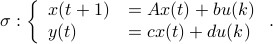
It is known that the input-output behaviour of any  , that is, the map from
  to
to  is invariant under a similarity transform.
To be explicit, the tuples
is invariant under a similarity transform.
To be explicit, the tuples  and
and 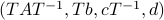 , which correspond to the change of coordinates
  for some
  , give rise to the same input-output behaviour.
Hence, one can define the equivalence relation
, give rise to the same input-output behaviour.
Hence, one can define the equivalence relation  by imposing that the input-output maps of and
  are equivalent.
By doing so we can consider the quotient
are equivalent.
By doing so we can consider the quotient  . However, in practice, given a , is any such that
  equally useful?
For example, the following and
equally useful?
For example, the following and  are similar, but clearly, is preferred from a numerical point of view:
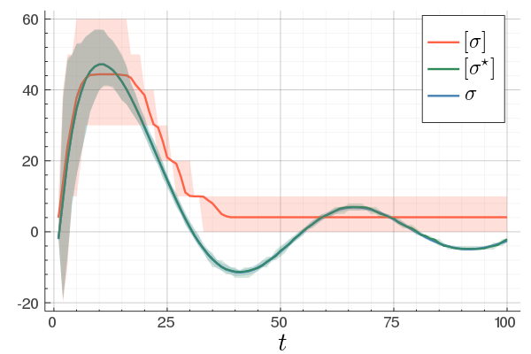
![A = left[begin{array}{ll} 0.5 & 10^9 0 & 0.5 end{array}right],quad A' = left[begin{array}{ll} 0.5 & 1 0 & 0.5 end{array}right].](eqs/6214495422406291774-130.png)
In what follows, we highlight the approach from Mullis and Roberts and conclude by how to optimally select . Norms will be interpreted in the  sense, that is, for
  ,
,  . Also, in what follows we assume that
  plus that is stable, which will mean
  and that corresponds to a minimal realization.
The first step is to quantify the error. Assume we have allocated  bits at our disposal to present the
  component of
  . These values for can differ, but we constrain the average by
  for some
  . Let
. Let  be a 'step-size’, such that our dynamic range of
  is bounded by
  (these are our possible representations). Next we use the modelling choices from Mullis and Roberts, of course, they are debatable, but still, we will infer some nice insights.
First, to bound the dynamic range, consider solely the effect of an input, that is, define  by
by 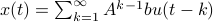 ,
, 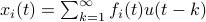 . Then we will impose the bound
  on . In combination with the step size (quantization), this results in
 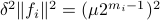 . Let
. Let  be a sequence of i.i.d. sampled random variables from
  . Then we see that
  . Hence, one can think of
  as scaling parameter related to the probability with which this dynamic range bound is true.
Next, assume that all the round-off errors are independent and have a variance of  .
Hence, the worst-case variance of computating
.
Hence, the worst-case variance of computating  is
is  . To evaluate the effect of this error on the output, assume for the moment that is identically .
Then,
. To evaluate the effect of this error on the output, assume for the moment that is identically .
Then,  . Similar to , define
  as the component of
  . As before we can compute the variance, this time of the full output signal, which yields
 . Note, these expressions hinge on the indepedence assumption.
Next, define the (infamous) matrices  ,
,  by
by
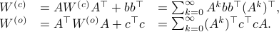
If we assume that the realization is not just minimal, but that  is a controllable pair and that
  is an observable pair, then,
  and
and  .
Now the key observation is that
.
Now the key observation is that  and similarly
  .
Hence, we can write
.
Hence, we can write  as
as  and indeed
  .
Using these Lyapunov equations we can say goodbye to the infinite-dimensional objects.
.
Using these Lyapunov equations we can say goodbye to the infinite-dimensional objects.
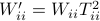
To combine these error terms, let say we have apply a coordinate transformation  , for some .
Specifically, let be diagonal and defined by
, for some .
Specifically, let be diagonal and defined by 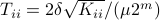 .
Then one can find that
.
Then one can find that 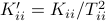 ,
,  . Where the latter expressions allows to express the output error (variance) by
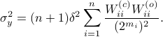
Now we want to minimize  over all plus some optimal selection of . At this point it looks rather painful. To make it work we first reformulate the problem using the well-known arithmetic-geometric mean inequality
![^{[1]}](eqs/2708305882951756665-130.png) for non-negative sequences
for non-negative sequences ![{a_i}_{iin [n]}](eqs/351138265746961916-130.png) :
:
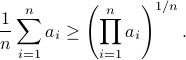
This inequality yields

See that the right term is independent of , hence this is a lower-bound with respect to minimization over . To achieve this (to make the inequality from an equality), we can select
Indeed, as remarked in the paper, is not per se an integer. Nevertheless, by this selection we find the clean expression from to minimize over systems equivalent to , that is, over some transformation matrix . Define a map ![f:mathcal{S}^n_{succ 0}to (0,1]](eqs/6462334851245421111-130.png) by
by
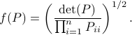
It turns out that  if and only if
  is diagonal. This follows
![^{[2]}](eqs/2708306882823756034-130.png) from Hadamard's inequality.
We can use this map to write
from Hadamard's inequality.
We can use this map to write

Since the term  is invariant under a transformation , we can only optimize over a structural change in realization tuple , that is, we need to make
  and
and  simultaneous diagonal! It turns out that this numerically 'optimal’ realization, denoted
  , is what is called a principal axis realization.
To compute it, diagonalize , 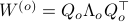 and define
 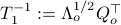 . Next, construct the diagonalization
 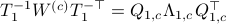 . Then our desired transformation is
  . First, recall that under any the pair
  becomes
 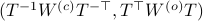 . Plugging in our map yields the transformed matrices
  , which are indeed diagonal.
 |
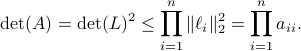
At last, we do a numerical test in Julia. Consider a linear system ![A = left[begin{array}{ll} 0.8 & 0.001 0 & -0.5 end{array} right],quad b = left[begin{array}{l} 10 0.1 end{array} right],](eqs/3623138148766993767-130.png)
![c=left[begin{array}{ll} 10 & 0.1 end{array} right],quad d=0.](eqs/42331078943303768-130.png)
To simulate numerical problems, we round the maps |
 and
and  to the closest integer where
 ![[cdot]](eqs/8251583936328055799-130.png) , naive realization
, naive realization ![[sigma]](eqs/4713363484184404481-130.png) and to the optimized one
and to the optimized one ![[sigma^{star}]](eqs/5091401033446485837-130.png) .
We do 100 experiments and show the mean plus the full confidence interval (of the input-output behaviour), the optimized representation is remarkably better.
Numerically we observe that for
.
We do 100 experiments and show the mean plus the full confidence interval (of the input-output behaviour), the optimized representation is remarkably better.
Numerically we observe that for  , which is precisely where the naive
 ![[1]](eqs/8209412804330245758-130.png) : To show this AM-GM inequality, we can use Jensen's inequality for concave functions, that is,
: To show this AM-GM inequality, we can use Jensen's inequality for concave functions, that is, ![mathbf{E}[g(x)]leq g(mathbf{E}[x])](eqs/8492979742681909343-130.png) . We can use the logarithm as our prototypical concave function on
. We can use the logarithm as our prototypical concave function on  and find
  . Then, the result follows.
![[2]](eqs/8209412804333245623-130.png) : The inequality attributed to Hadamard is slightly more difficult to show. In its general form the statement is that
: The inequality attributed to Hadamard is slightly more difficult to show. In its general form the statement is that 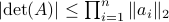 , for
, for  the column of . The inequality becomes an equality when the columns are mutually orthogonal. The intuition is clear if one interprets the determinant as the signed volume spanned by the columns of , which. In case
  , we know that there is
  such that
  , hence, by this simple observation it follows that
Equality holds when the columns are orthogonal, so  must be diagonal, but
  must also hold, hence,
  must be diagonal, and thus must be diagonal, which is the result we use.
Spectral Radius vs Spectral Norm |28 Febr. 2020|
tags: math.LA, math.DS
Lately, linear discrete-time control theory has start to appear in areas far beyond the ordinary. As a byproduct, papers start to surface which claim that stability of linear discrete-time systems

is characterized by  .
The confunsion is complete by calling this object the spectral norm of a matrix .
Indeed, stability of is not characterized by
.
The confunsion is complete by calling this object the spectral norm of a matrix .
Indeed, stability of is not characterized by  , but by
 ![rho(A):=max_{iin [n]}|lambda_i(A)|](eqs/8716262940618826552-130.png) .
If , then all absolute eigenvalues of are strictly smaller than one, and hence for
.
If , then all absolute eigenvalues of are strictly smaller than one, and hence for  ,
,  .
This follows from the Jordan form of in combination with the simple observation that for
.
This follows from the Jordan form of in combination with the simple observation that for  ,
,  .
.
To continue, define two sets;  and
and  .
Since
.
Since  we have
  . Now, the main question is, how much do we lose by approximating
  with
with  ? Motivation to do so is given by the fact that
  is a norm and hence a convex function, i.e., when given a convex polytope
  with vertices
  , if
, if  , then
  . Note that
  is not a norm, can be without
  (consider an upper-triangular matrix with zeros on the main diagonal), the triangle inequality can easily fail as well. For example, let
![A_1 = left[begin{array}{ll} 0 & 1 0 & 0 end{array}right], quad A_2 = left[begin{array}{ll} 0 & 0 1 & 0 end{array}right],](eqs/6730715665771009175-130.png)
Then  , but
, but  , hence
  fails to hold.
A setting where the aforementioned property of might help is Robust Control, say we want to assess if some algorithm rendered a compact convex set , filled with 's, stable.
As highlighted before, we could just check if all extreme points of are members of
fails to hold.
A setting where the aforementioned property of might help is Robust Control, say we want to assess if some algorithm rendered a compact convex set , filled with 's, stable.
As highlighted before, we could just check if all extreme points of are members of  , which might be a small and finite set.
Thus, computationally, it appears to be attractive to consider over the generic .
, which might be a small and finite set.
Thus, computationally, it appears to be attractive to consider over the generic .
As a form of critique, one might say that is a lot larger than .
Towards such an argument, one might recall that  . Indeed,
  if
if![^{[3]}](eqs/2708307882947756447-130.png)
 , but
, but  . Therefore, it seems like the set of for which considering over
  is reasonable, is negligibly small.
To say a bit more, since
is reasonable, is negligibly small.
To say a bit more, since![^{[4]}](eqs/2708308882819756064-130.png)
 we see that we can always find a ball with non-zero volume fully contained in .
Hence, is at least locally dense in
we see that we can always find a ball with non-zero volume fully contained in .
Hence, is at least locally dense in  . The same holds for
  (which is more obvious).
So in principle we could try to investigate
(which is more obvious).
So in principle we could try to investigate  . For
. For  , the sets agree, which degrades asymptotically.
However, is this the way to go? Lets say we consider the set
, the sets agree, which degrades asymptotically.
However, is this the way to go? Lets say we consider the set  . Clearly, the sets
  and are different, even in volume, but for sufficiently large
  , should we care? The behaviour they parametrize is effectively the same.
We will stress that by approximating  with , regardless of their volumetric difference, we are ignoring a full class of systems and miss out on a non-neglible set of behaviours.
To see this, any system described by is contractive in the sense that
with , regardless of their volumetric difference, we are ignoring a full class of systems and miss out on a non-neglible set of behaviours.
To see this, any system described by is contractive in the sense that  , while systems in are merely asymptotically stable. They might wander of before they return, i.e., there is no reason why for all
  we must have
  . We can do a quick example, consider the matrices
![A_2 = left[begin{array}{lll} 0 & -0.9 & 0.1 0.9 & 0 & 0 0 & 0 & -0.9 end{array}right], quad A_{rho} = left[begin{array}{lll} 0.1 & -0.9 & 1 0.9 & 0 & 0 0 & 0 & -0.9 end{array}right].](eqs/7939256391259616851-130.png)
Then  ,
,  and both
  and
and  have
have  .
We observe that indeed is contractive, for any initial condition on
.
We observe that indeed is contractive, for any initial condition on  , we move strictly inside the sphere, whereas for , when starting from the same initial condition, we take a detour outside of the sphere before converging to . So although and have the same spectrum, they parametrize different systems.
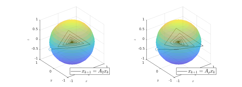 |
In our deterministic setting this would mean that we would confine our statespace to a (solid) sphere with radius  , instead of .
Moreover, in linear optimal control, the resulting closed-loop system is usually not contractive.
Think of the infamous pendulum on a cart. Being energy efficient has usually nothing to do with taking the shortest, in the Euclidean sense, path.
, instead of .
Moreover, in linear optimal control, the resulting closed-loop system is usually not contractive.
Think of the infamous pendulum on a cart. Being energy efficient has usually nothing to do with taking the shortest, in the Euclidean sense, path.
: Recall,  . Then, let
  be some eigenvector of . Now we have
  . Since this eigenvalue is arbitrary it follows that
  .
.
: Let  then
then  . This follows from the being a norm.
![[3]](eqs/8209412804332245752-130.png) : Clearly, if , we have
: Clearly, if , we have  . Now, when
  , does this imply that ? The answer is no, consider
![A' = left[begin{array}{lll} 0.9 & 0 & 0 0 & 0.1 & 0 0 & 0.1 & 0.1 end{array}right].](eqs/1479234184051328788-130.png)
Then,  , yet,
  . For the full set of conditions on such that see this paper by Goldberg and Zwas.
![[4]](eqs/8209412804335245617-130.png) : Recall that
: Recall that  . This expression is clearly larger or equal to
  .
.
A Special Group, Volume Preserving Feedback |16 Nov. 2019|
tags: math.LA, math.DS
This short note is inspired by the beautiful visualization techniques from Duistermaat and Kolk (DK1999).
Let's say we have a  -dimensional linear discrete-time dynamical system
  , which preserves the volume of the cube
 ![[-1,1]^2](eqs/7220646983027292775-130.png) under the dynamics, i.e.
under the dynamics, i.e. ![mathrm{Vol}([-1,1]^2)=mathrm{Vol}(A^k[-1,1]^2)](eqs/6078350520623442645-130.png) for any
for any  .
.
Formally put, this means that is part of a certain group, specifically, consider some field  and
define the Special Linear group by
and
define the Special Linear group by

Now, assume that we are only interested in matrices 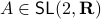 such that the cube remains bounded under the dynamics, i.e.,
 ![lim_{kto infty}A^k[-1,1]^2](eqs/6180125548835686349-130.png) is bounded. In this scenario we restrict our attention to
is bounded. In this scenario we restrict our attention to 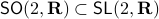 . To see why this is needed, consider
  and both with determinant :
![A_1 = left[ begin{array}{ll} 2 & 0 0 & frac{1}{2} end{array}right], quad A_2 = left[ begin{array}{ll} 1 & 2 0 & 1 end{array}right],](eqs/4004660008936570769-130.png)
If we look at the image of under both these maps (for several iterations), we see that volume is preserved, but also clearly that the set is extending indefinitely in the horizontal direction.
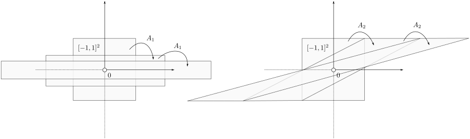 |
To have a somewhat interesting problem, assume we are given  with
with  while it is our task to find a
  such that
  , hence, find feedback which not only preserves the volume, but keeps any set of initial conditions (say ) bounded over time.
Towards a solution, we might ask, given any what is the nearest (in some norm) rotation matrix? This turns out to be a classic question, starting from orthogonal matrices, the solution to  is given by
  , where
  follows from the SVD of ,
  .
Differently put, when we use a polar decomposition of ,
.
Differently put, when we use a polar decomposition of ,  , then the solution is given by
  . See this note for a quick multiplier proof.
An interesting sidenote, problem is well-defined since
. See this note for a quick multiplier proof.
An interesting sidenote, problem is well-defined since  is compact. To see this, recall that for any
  we have
  , hence the set is bounded, plus is the pre-image of
  under
under  ,
,  , hence the set is closed as well.
This is great, however, we would like to optimize over  instead. To do so, one usually resorts to simply checking the sign - and if necessary - flipping it via finding the closest matrix with a change in determinant sign.
We will see that by selecting appropriate coordinates we can find the solution without this checking of signs.
instead. To do so, one usually resorts to simply checking the sign - and if necessary - flipping it via finding the closest matrix with a change in determinant sign.
We will see that by selecting appropriate coordinates we can find the solution without this checking of signs.
For today we look at  and largely follow (DK1999), for such a -dimensional matrix, the determinant requirement translates to
  . Under the following (invertible) linear change of coordinates
![left[ begin{array}{l} a d b c end{array}right] = left[ begin{array}{llll} 1 & 1 & 0 & 0 1 & -1 & 0 & 0 0 & 0 & 1 & 1 0 & 0 & 1 & -1 end{array}right] left[ begin{array}{l} p q r s end{array}right]](eqs/6118233270205082065-130.png)
 becomes
  , i.e., for any pair
  the point
  runs over a circle with radius
  . Hence, we obtain the diffeomorphism
  . We can use however a more pretty diffeomorphism of the sphere and an open set in . To that end, use the diffeomorphism:
![(theta,(u,v)) mapsto frac{1}{sqrt{1-u^2-v^2}} left[ begin{array}{ll} cos(theta)+u & -sin(theta)+v sin(theta)+v & cos(theta)-u end{array}right] in mathsf{SL}(2,mathbf{R}),](eqs/6656969251929689946-130.png)
for  (formal way of declaring that
  should not be any real number) and the pair
  being part of
  (the open unit-disk).
To see this, recall that the determinant is not a linear operator.
Since we have a -dimensional example we can explicitly compute the eigenvalues of any (plug into the characteristic equation) and obtain:
(the open unit-disk).
To see this, recall that the determinant is not a linear operator.
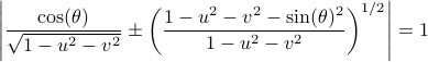
Since we have a -dimensional example we can explicitly compute the eigenvalues of any (plug into the characteristic equation) and obtain:
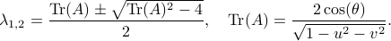
At this point, the only demand on the eigenvalues is that  . Therefore, when we would consider within the context of a discrete linear dynamical system , is either a saddle-point, or we speak of a marginally stable system (
 ).
We can visualize the set of all marginally stable , called
).
We can visualize the set of all marginally stable , called  , defined by all
 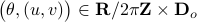 satisfying
(DK1999) J.J. Duistermaat and J.A.C. Kolk : ‘‘Lie Groups’’, 1999 Springer.
Riemannian Gradient Flow |5 Nov. 2019|
tags: math.DG, math.DS
Previously we looked at  ,
,  - and its resulting flow - as the result from mapping to the sphere. However, we saw that for
  this flow convergences to
  , with
 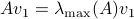 such that for
  we have
 . Hence, it is interesting to look at the flow from an optimization point of view:
  .
.
A fair question would be, is our flow not simply Riemannian gradient ascent for this problem? As common with these kind of problems, such a hypothesis is something you just feel.
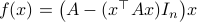
Now, using the tools from (CU1994, p.311) we can compute the gradient of  (on the sphere) via
  , where
  is a vector field normal to , e.g.,
  .
From there we obtain
.
From there we obtain
![mathrm{grad}_{mathbf{S}^2}(g|_{mathbf{S}^2}) = left[ begin{array}{lll} (1-x^2) & -xy & -xz -xy & (1-y^2) & -yz -xz & -yz & (1-z^2) end{array}right] left[ begin{array}{l}partial_x g partial_y g partial_z g end{array}right]=G(x,y,z)nabla g.](eqs/2499009703266316151-130.png)
To make our life a bit easier, use instead of the map  . Moreover, set
  . Then it follows that
![begin{array}{ll} mathrm{grad}_{mathbf{S}^2}(h|_{mathbf{S}^2}) &= left(I_3-mathrm{diag}(s)left[begin{array}{l} s^{top}s^{top}s^{top} end{array}right]right) 2A^{top}As &= 2left(A^{top}A-(s^{top}A^{top}Asright)I_3)s. end{array}](eqs/2245781100057659571-130.png)
Of course, to make the computation cleaner, we changed to  , but the relation between
  and is beautiful. Somehow, mapping trajectories of , for some , to the sphere corresponds to (Riemannian) gradient ascent applied to the problem
  .
.
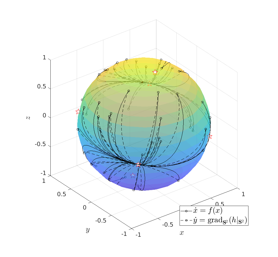 |
To do an example, let ![A = left[ begin{array}{lll} 10 & 2 & 0 2 & 10 & 2 0 & 2 & 1 end{array}right].](eqs/6133576945654762450-130.png)
We can compare |
 be given by
 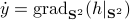 . We see that the gradient flow under the quadratic function takes a clearly ‘‘shorter’’ path.
 Now, we formalize the previous analysis a bit a show how fast we convergence. Assume that the eigenvectors are ordered such that eigenvector  corresponds to the largest eigenvalue of . Then, the solution to
 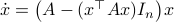 is given by
Let  be
be  expressed in eigenvector coordinates, with all
  (normalized). Moreover, assume all eigenvalues are distinct. Then, to measure if is near , we compute
  , which is if and only if is parallel to . To simplify the analysis a bit, we look at
  , for some perturbation
  , this yields
Next, take the the (natural) logarithm on both sides:
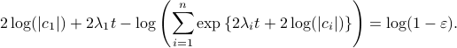
This log-sum-exp terms are hard to deal with, but we can apply the so-called ‘‘log-sum-exp trick’’:

In our case, we set  and obtain
![-log left(sum^{n}_{i=1}exp left{2 left[(lambda_i-lambda_1)t + logleft(frac{|c_i|}{|c_1|} right) right] right}+1 right) = log(1-varepsilon).](eqs/3165375830294523712-130.png)
We clearly observe that for  the LHS approaches from below, which means that
  from above, like intended. Of course, we also observe that the mentioned method is not completely general, we already assume distinct eigenvalues, but there is more. We do also not convergence when
  , which is however a set of measure on the sphere .
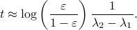
More interestingly, we see that the convergence rate is largely dictated by the ‘‘spectral gap/eigengap’’  . Specifically, to have a particular projection error
  , such that
  , we need
Comparing this to the resulting flow from  ,
,  , we see that we have the same flow, but with
  .
This is interesting, since and
.
This is interesting, since and  have the same eigenvectors, yet a different (scaled) spectrum. With respect to the convergence rate, we have to compare
  and
and  for any
  with
with  (the additional is not so interesting).
It is obvious what we will happen, the crux is, is  larger or smaller than ? Can we immediately extend this to a Newton-type algorithm? Well, this fails (globally) since we work in instead of purely with . To be concrete,
  , we never have degrees of freedom.
Of course, these observations turned out to be far from new, see for example (AMS2008, sec. 4.6).
(AMS2008) P.A. Absil, R. Mahony and R. Sepulchre: ‘‘Optimization Algorithms on Matrix Manifolds’’, 2008 Princeton University Press.
(CU1994) Constantin Udriste: ‘‘Convex Functions and Optimization Methods on Riemannian Manifolds’’, 1994 Kluwer Academic Publishers.
Dynamical Systems on the Sphere |3 Nov. 2019|
tags: math.DS
 |
In this post we start a bit with control of systems living on compact metric spaces. This is interesting since we have to rethink what we want, |
 cannot even occur.
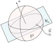
Let a great arc (circle)
cannot even occur.
Let a great arc (circle)  on
on  be parametrized by the normal of a hyperplane
  through
  ,
,  is the axis of rotation for
 To start, consider a linear dynamical systems ,  , for which the solution is given by
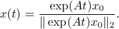
 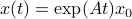 . We can map this solution to the sphere via
  .
The corresponding vector field for is given by
.
The corresponding vector field for is given by
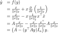
The beauty is the following, to find the equilibria, consider 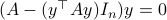 . Of course,
  is not valid since
  . However, take any eigenvector
  of , then
  is still an eigenvector, plus it lives on . If we plug such a scaled (from now on consider all eigenvectors to live on ) into
  we get
  , which is rather cool. The eigenvectors of are (at least) the equilibria of
  . Note, if
  , then so is
  , each eigenvector gives rise to two equilibria.
We say at least, since if
, each eigenvector gives rise to two equilibria.
We say at least, since if  is non-trivial, then for any
  , we get
  .
.
Let  , then what can be said about the stability of the equilibrium points?
Here, we must look at
, then what can be said about the stability of the equilibrium points?
Here, we must look at  , where the -dimensional system is locally a
  -dimensional linear system. To do this, we start by computing the standard Jacobian of , which is given by

As said before, we do not have a -dimensional system. To that end, we assume  with diagonalization
  (otherwise peform a Gram-Schmidt procedure) and perform a change of basis
  . Then if we are interested in the qualitative stability properties of
  (the eigenvector of ), we can simply look at the eigenvalues of the matrix resulting from removing the row and column in
  , denoted
  .
.
We do two examples. In both figures are the initial conditions indicated with a dot while the equilibrium points are stars.
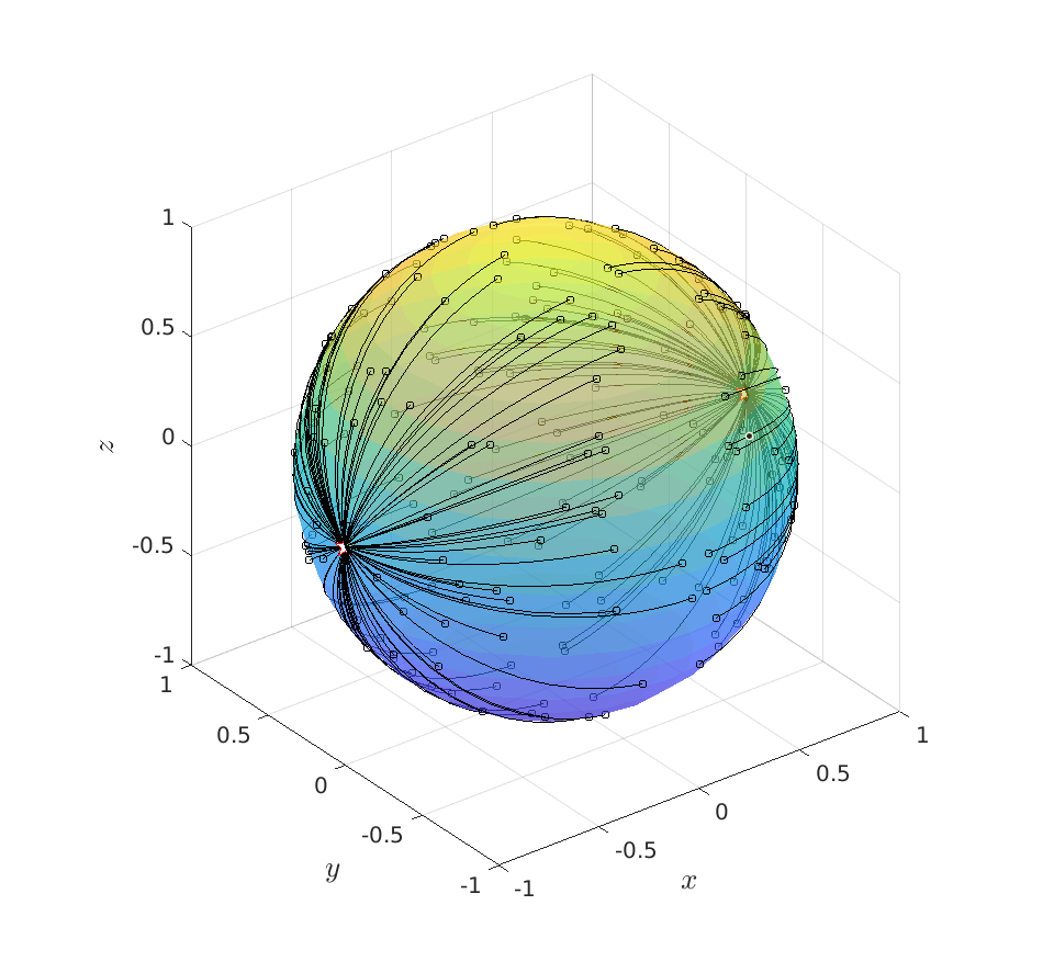 |
First, let ![A_1 = left[ begin{array}{lll} 1 & 0 & 0 0 & -1 & 0 0 & 0 & -1 end{array}right]](eqs/4948366788842116208-130.png)
Clearly, for |
 and let
  be
be  . Then using the procedure from before, we find that
  are locally unstable in one direction while
 Finite Calls to Stability | 31 Oct. 2019 |
tags: math.LA, math.DS
Consider an unknown dynamical system parametrized by .
In this short note we look at a relatively simple, yet neat method to assess stability of via finite calls to a particular oracle. Here, we will follow the notes by Roman Vershynin (RV2011).
Assume we have no knowledge of , but we are able to obtain  for any desired
  . It turns out that we can use this oracle to bound from above.
First, recall that since is symmetric,  . Now, the common definition of
  is
is  . The constraint set is not per se convenient from a computational point of view. Instead, we can look at a compact constraint set:
 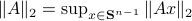 , where is the sphere in .
The latter formulation has an advantage, we can discretize these compact constraints sets and tame functions over the individual chunks.
, where is the sphere in .
The latter formulation has an advantage, we can discretize these compact constraints sets and tame functions over the individual chunks.
To do this formally, we can use -nets, which are convenient in quantitative analysis on compact metric spaces  . Let
. Let  be a -net for if
  . Hence, we measure the amount of balls to cover .
For example, take  as our metric space where we want to bound
  (the cardinality, i.e., the amount of balls). Then, to construct a minimal set of balls, consider an -net of balls
  , with
  . Now the insight is simply that
  .
Luckily, we understand the volume of -dimensional Euclidean balls well such that we can establish
.
Luckily, we understand the volume of -dimensional Euclidean balls well such that we can establish

Which is indeed sharper than the bound from Lemma 5.2 in (RV2011).
Next, we recite Lemma 5.4 from (RV2011). Given an -net for with  we have
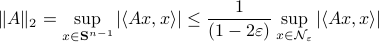
This can be shown using the Cauchy-Schwartz inequality. Now, it would be interesting to see how sharp this bound is.
To that end, we do a -dimensional example ( ). Note, here we can easily find an optimal grid using polar coordinates. Let the unknown system be parametrized by
![A = left[ begin{array}{ll} 0.1 & -0.75 -0.75 & 0.1 end{array}right]](eqs/8870555444473195760-130.png)
such that  . In the figures below we compute the upper-bound to for several nets
  .
Indeed, for finer nets, we see the upper-bound approaching
.
Indeed, for finer nets, we see the upper-bound approaching  . However, we see that the convergence is slow while being inversely related to the exponential growth in .
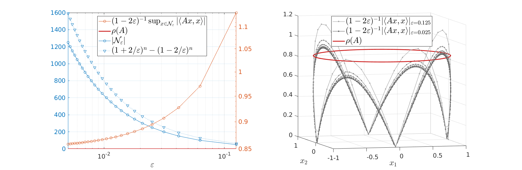 |
Overall, we see that after about a 100 calls to our oracle we can be sure about being exponentially stable.
Here we just highlighted an example from (RV2011), at a later moment we will discuss its use in probability theory.