Topological Considersations in Stability Analysis |17 November 2020|
tags: math.DS
In this post we discuss very classical, yet, highly underappreciated topological results.
We will look at dynamical control systems of the form

where  is some finite-dimensional embedded manifold.
As it turns out, topological properties of encode a great deal of fundamental control possibilities, most notably, if a continuous globally asymptotically stabilizing control law exists or not (usually, one can only show the negative). In this post we will work towards two things, first, we show that a technically interesting nonlinear setting is that of a dynamical system evolving on a compact manifold, where we will discuss that the desirable continuous feedback law can never exist, yet, the boundedness implied by the compactness does allow for some computations. Secondly, if one is determined to work on systems for which a continuous globally asymptotically stable feedback law exists, then a wide variety of existential sufficient conditions can be found, yet, the setting is effectively Euclidean, which is the most basic nonlinear setting.
To start the discussion, we need one important topological notion.
Definition [Contractability].
Given a topological manifold  . If the map
  is null-homotopic, then, is contractible.
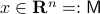
To say that a space is contractible when it has no holes (genus  ) is wrong, take for example the sphere. The converse is true, any finite-dimensional space with a hole cannot be contractible. See Figure 1 below.
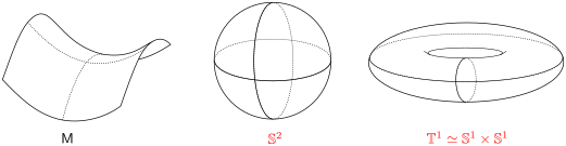 |
Figure 1:
The manifold |
 and
and Topological Obstructions to Global Asymptotic Stability
In this section we highlight a few (not all) of the most elegant topological results in stability theory. We focus on results without appealing to the given or partially known vector field  .
This line of work finds its roots in work by Bhatia, Szegö, Wilson, Sontag and many others.
.
This line of work finds its roots in work by Bhatia, Szegö, Wilson, Sontag and many others.
Theorem [The domain of attraction is contractible, Theorem 21]
Let the flow  be continuous and let
  be an asymptotically stable equilibrium point. Then, the domain of attraction
  is contractible.
This theorem by Sontag states that the underlying topology of a dynamical system, better yet, the space on which the dynamical system evolves, dictates what is possible. Recall that linear manifolds are simply hyperplanes, which are contractible and hence, as we all know, global asymptotic stability is possible for linear systems. However, if is not contractible, there does not exist a globally asymptotically stabilizable continuous-time system on , take for example any sphere.
The next example shows that one should not underestimate ‘‘linear systems’’ either.
Example [Dynamical Systems on  ]
Recall that
]
Recall that  is a smooth
  -dimensional manifold (Lie group).
Then, consider for some
-dimensional manifold (Lie group).
Then, consider for some  ,
,  the (right-invariant) system

Indeed, the solution to (1) is given by  . Since this group consists out of two disjoint components there does not exist a matrix
  , or continuous nonlinear map for that matter, which can make a vector field akin to (1) globally asymptotically stable. This should be contrasted with the closely related ODE
  ,
,  . Even for the path connected component
  , The theorem by Sontag obstructs the existence of a continuous global asymptotically stable vector field. This because the group is not simply connected for (This follows most easily from establishing the homotopy equivalence between
  and
and  via (matrix) Polar Decomposition), hence the fundamental group is non-trivial and contractibility is out of the picture. See that if one would pick to be stable (Hurwitz), then for
  we have
 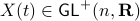 , however
  .
.
Following up on Sontag, Bhat and Bernstein revolutionized the field by figuring out some very important ramifications (which are easy to apply). The key observation is the next lemma (that follows from intersection theory arguments, even for non-orientable manifolds).
Lemma [Proposition 1] Compact, boundaryless, manifolds are never contractible.
Clearly, we have to ignore -dimensional manifolds here. Important examples of this lemma are the  -sphere
  and the rotation group
  as they make a frequent appearance in mechanical control systems, like a robotic arm.
Note that the boundaryless assumption is especially critical here.
as they make a frequent appearance in mechanical control systems, like a robotic arm.
Note that the boundaryless assumption is especially critical here.
Now the main generalization by Bhat and Bernstein with respect to the work of Sontag is to use a (vector) bundle construction of .
Loosely speaking, given a base  and total manifold , is a vector bundle when for the surjective map
  and each
  we have that the fiber
  is a finite-dimensional vector space (see the great book by Abraham, Marsden and Ratiu Section 3.4 and/or the figure below).
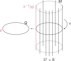 |
Figure 2:
A prototypical vector bundle, in this case the cylinder |
Intuitively, vector bundles can be thought of as manifolds with vector spaces attached at each point, think of a cylinder living in  , where the base manifold is
  and each fiber is a line through
  extending in the third direction, as exactly what the figure shows. Note, however, this triviality only needs to hold locally.
A concrete example is a rigid body with  , for which a large amount of papers claim to have designed continuous globally asymptotically stable controllers. The fact that this was so enormously overlooked makes this topological result not only elegant from a mathematical point of view, but it also shows its practical value.
The motivation of this post is precisely to convey this message, topological insights can be very fruitful.
, for which a large amount of papers claim to have designed continuous globally asymptotically stable controllers. The fact that this was so enormously overlooked makes this topological result not only elegant from a mathematical point of view, but it also shows its practical value.
The motivation of this post is precisely to convey this message, topological insights can be very fruitful.
Now we can state their main result
Theorem [Theorem 1]
Let  be a compact, boundaryless, manifold, being the base of the vector bundle
  with
with  , then, there is no continuous vector field on with a global asymptotically stable equilibrium point.
Indeed, compactness of can also be relaxed to not being contractible as we saw in the example above, however, compactness is in most settings more tangible to work with.
Example [The Grassmannian manifold]
The Grassmannian manifold, denoted by  , is the set of all
  -dimensional subspaces
  . One can identify with the Stiefel manifold
  , the manifold of all orthogonal -frames, in the bundle sense of before, that is
  such that the fiber
  represent all -frames generating the subspace
  . In its turn, can be indentified with the compact Lie group
  (via a quotient), such that indeed is compact.
This manifold shows up in several optimization problems and from our continuous-time point of view we see that one can never find, for example, a globally converging gradient-flow like algorithm.
(via a quotient), such that indeed is compact.
This manifold shows up in several optimization problems and from our continuous-time point of view we see that one can never find, for example, a globally converging gradient-flow like algorithm.
Example [Tangent Bundles]
By means of a Lagrangian viewpoint, a lot of mechanical systems are of a second-order nature, this means they are defined on the tangent bundle of some , that is,  . However, then, if the configuration manifold is compact, we can again appeal to the Theorem by Bhat and Bernstein. For example, Figure 2 can relate to the manifold over which the pair
  is defined.
Global Isomorphisms
One might wonder, given a vector field  over a manifold , since we need contractibility of for to have a global asymptotically stable equilibrium points, how interesting are these manifolds? As it turns out, for
  , which some might call the high-dimensional topological regime, contractible manifolds have a particular structure.
A topological space being simply connected is equivalent to the corresponding fundamental group being trivial. However, to highlight the work by Stallings, we need a slightly less well-known notion.
Definition [Simply connected at infinity]
The topological space is simply connected at infinity, when for any compact subset  there exists a
  where
where  such that
  is simply connected.
This definition is rather complicated to parse, however, we can give a more tangible description. Let be a non-compact topological space, then, is said to have one end when for any compact  there is a where such that is connected. So,
  , as expected, fails to have one end, while
  does have one end.
Now, Proposition 2.1 shows that if and
does have one end.
Now, Proposition 2.1 shows that if and  are simply connected and both have one end, then
  is simply connected at infinity. This statement somewhat clarifies why dimension
  and above are somehow easier to parse in the context of topology. A similar statement can be made about the cylindrical space
  .
.
Lemma [Product representation Proposition 2.4]
Let and be manifolds of dimension greater or equal than  . If
. If  is contractible and
  , then, is simply connected at infinity.
Now, most results are usually stated in the context of a piecewise linear (PL) topology. By appealing to celebrated results on triangulization (by Whitehead) we can state the following.
Theorem [Global diffeomorphism Theorem 5.1]
Let be a contractible  ,
,  , -dimensional manifold which is simply connected at infinity. If , then, is diffeomorphic to
  .
.
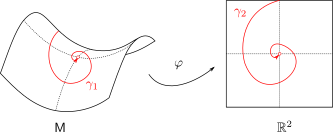 |
Figure 3:
The manifold |
 is usually much easier than dealing with
  directly.
 You might say that this is all obvious, as in Figure 3, we can always do it, also for lower-dimensions. However, there is famous counterexample by Whitehead, which provided lots of motivation for the community:
‘‘There is an open,  -dimensional manifold which is contractible, but not homeomorphic to .’’
In fact, this example was part of the now notorious program to solve the Poincaré conjecture. All in all, this shows that contractible manifolds are not that interesting from a nonlinear dynamical systems point of view, compact manifolds is a class of manifolds providing for more of a challenge.
Remark on the Stabilization of Sets
So far, the discussion has been on the stabilization of (equilibrium) points, now what if we want to stabilize a curve or any other desirable set, that is, a non-trivial set  . It seems like the shape of these objects, with respect to the underlying topology of , must indicate if this is possible again? Let
  denote an open neighbourhood of some
  . In what follows, the emphasis is on
  and having the same topology. We will be brief and follow Moulay and Bhat.
Lemma [Theorem 5]
Consider a closed-loop dynamical system given rise to a continuous flow. Suppose that the compact set  is asymptotically stable with domain of attraction
  . Then, is a weak deformation retract of
  .
.
In rather loose terms, being a weak deformation retract of means that one can continuously ‘‘retract’’ points from and morph them into the set . So, this works for and  , due to being punctured. See p.200 for more information on retracts. In Figure 4 below we show that since this lemma is mostly concerned with the local topology, the global topology is less important. For , the set is not a deformation retract of the set
  such that can never be a region of attraction, this should be contrasted with the setting on the Torus
  .
.
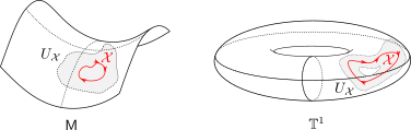 |
Figure 4:
The topological relation between |
The beauty of all of this is that even if you are not so sure about the exact dynamical system at hand, the underlying topology can already provide for some answers. In particular, to determine, what can, or cannot be done.
This post came about during a highly recommended course at EPFL.