Posts (9) containing the 'math.LA’ (Linear Algebra) tag:
On the complexity of matrix multiplications |10 October 2022|
tags: math.LA
Recently, DeepMind published new work on ‘‘discovering’’ numerical linear algebra routines. This is remarkable, but I leave the assesment of this contribution to others. Rather, I like to highlight the earlier discovery of Strassen. Namely, how to improve upon the obvious matrix multiplication algorithm.
To get some intuition, consider multiplying two complex numbers  , that is, construct
  . In this case, the obvious thing to do would lead to 4 multiplications, namely
  ,
,  ,
,  and
and  . However, consider using only
  , and . These multiplications suffice to construct
  (subtract the latter two from the first one). The emphasis is on multiplications as it seems to be folklore knowledge that multiplications (and especially divisions) are the most costly. However, note that we do use more additive operations. Are these operations not equally ‘‘costly’’? The answer to this question is delicate and still changing!
When working with integers, additions are indeed generally ‘‘cheaper’’ than multiplications. However, oftentimes we work with floating points. Roughly speaking, these are numbers  characterized by some (signed) mantissa
  , a base
  and some (signed) exponent
  , specifically,
  . For instance, consider the addition
  . To perform the addition, one normalizes the two numbers, e.g., one writes
  . Then, to perform the addition one needs to take the appropriate precision into account, indeed, the result is
  . All this example should convey is that we have sequential steps. Now consider multiplying the same numbers, that is,
  . In this case, one can proceed with two steps in parallel, on the one hand
  and on the other hand
  . Again, one needs to take the correct precision into account in the end, but we see that by no means multiplication must be significantly slower in general!
Now back to the matrix multiplication algorithms. Say we have
![A = left[begin{array}{ll} A_{11} & A_{12} A_{21} & A_{22} end{array}right],quad B = left[begin{array}{ll} B_{11} & B_{12} B_{21} & B_{22} end{array}right],](eqs/6805404554309501197-130.png)
then,  is given by
![C = left[begin{array}{ll} C_{11} & C_{12} C_{21} & C_{22} end{array}right]= left[begin{array}{ll} A_{11}B_{11}+A_{12}B_{21} & A_{11}B_{12}+A_{12}B_{22} A_{21}B_{11}+A_{22}B_{21} & A_{21}B_{12}+A_{22}B_{22} end{array}right].](eqs/6225513400863626014-130.png)
Indeed, the most straightforward matrix multiplication algorithm for  and
and  costs you
  multiplications and
  additions.
Using the intuition from the complex multiplication we might expect we can do with fewer multiplications. In 1969 (Numer. Math. 13 354–356) Volker Strassen showed that this is indeed true.
additions.
Using the intuition from the complex multiplication we might expect we can do with fewer multiplications. In 1969 (Numer. Math. 13 354–356) Volker Strassen showed that this is indeed true.
Following his short, but highly influential, paper, let  ,
,  ,
,  ,
, 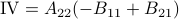 ,
, 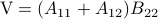 ,
,  and
and  . Then,
  ,
, 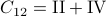 ,
, 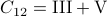 and
and  .
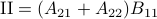
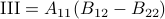
See that we need
.
See that we need  multiplications and
  additions to construct
  for both
  and
and  being
being  -dimensional. The ‘‘obvious’’ algorithm would cost
  multiplications and
  additions. Indeed, one can show now that for matrices of size
  one would need
  multiplications (via induction). Differently put, one needs
  multiplications.
This bound prevails when including all operations, but only asymptotically, in the sense that
multiplications.
This bound prevails when including all operations, but only asymptotically, in the sense that  . In practical algorithms, not only multiplications, but also memory and indeed additions play a big role. I am particularly interested how the upcoming DeepMind algorithms will take numerical stability into account.
*Update: the improved complexity got immediately improved.
Endomorphisms, Tensors in Disguise |18 August 2020|
tags: math.LA
Unfortunately the radio silence remained, the good news is that even more cool stuff is on its way*!
For now, we briefly mention a very beautiful interpretation of  -tensors.
Given some vectorspace
-tensors.
Given some vectorspace  , let
, let  be the set of linear endomorphisms from to .
Indeed, for finite-dimensional vector spaces one can just think of these maps as being parametrized by matrices.
Now, we recall that -tensors are multilinear maps which take an element of and its dual space
be the set of linear endomorphisms from to .
Indeed, for finite-dimensional vector spaces one can just think of these maps as being parametrized by matrices.
Now, we recall that -tensors are multilinear maps which take an element of and its dual space  and map it some real number, that is,
  .
.
The claim is that for finite-dimensional the set is isomorphic to the set of -tensors  . This is rather intuitive to see, let
  and
and  , then, we can write
  and think of
  as a matrix. This can be formalized, as is done here by showing there is a bijective map
  .
So, we can identify any
.
So, we can identify any  with some , that is
  . Similarly, we can fix
  and identify with a linear map in the dual space, that is
  . Regardless, both represent the same tensor evaluation, hence
which is indeed the standard dual map definition.
Now we use this relation, recall that discrete-time linear systems are nothing more then maps  , that is, linear endomorphims, usually on
  . Using the tensor interpretation we recover what is sometimes called the ‘‘dual system’’ to , namely
  (suggestive notation indeed). Using more traditional notation for the primal:
  and dual:
 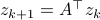 system, we recover that
  . Then, let
  and
and  for
for  and
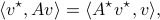
and  being left- and right-eigenvector of , respectively. We see that this implies that
 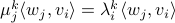 , for
, for  the eigenvalue corresponding to and
  the eigenvalue corresponding to . Hence, in general, the eigenspaces of and
  are generically orthogonal.
In other words, we recover the geometric interpretation of mapping  -volumes under versus
* See this talk by Daniel.
Optimal coordinates |24 May 2020|
tags: math.LA, math.OC, math.DS
There was a bit of radio silence, but as indicated here, some interesting stuff is on its way.
In this post we highlight this 1976 paper by Mullis and Roberts on ’Synthesis of Minimum Roundoff Noise Fixed Point Digital Filters’.
Let us be given some single-input single-output (SISO) dynamical system 
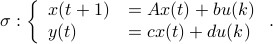
It is known that the input-output behaviour of any  , that is, the map from
  to
to  is invariant under a similarity transform.
To be explicit, the tuples
is invariant under a similarity transform.
To be explicit, the tuples  and
and  , which correspond to the change of coordinates
  for some
  , give rise to the same input-output behaviour.
Hence, one can define the equivalence relation
, give rise to the same input-output behaviour.
Hence, one can define the equivalence relation  by imposing that the input-output maps of and
  are equivalent.
By doing so we can consider the quotient
are equivalent.
By doing so we can consider the quotient  . However, in practice, given a , is any such that
  equally useful?
For example, the following and
equally useful?
For example, the following and  are similar, but clearly, is preferred from a numerical point of view:
![A = left[begin{array}{ll} 0.5 & 10^9 0 & 0.5 end{array}right],quad A' = left[begin{array}{ll} 0.5 & 1 0 & 0.5 end{array}right].](eqs/6214495422406291774-130.png)
In what follows, we highlight the approach from Mullis and Roberts and conclude by how to optimally select . Norms will be interpreted in the  sense, that is, for
  ,
,  . Also, in what follows we assume that
  plus that is stable, which will mean
  and that corresponds to a minimal realization.
The first step is to quantify the error. Assume we have allocated  bits at our disposal to present the
  component of
  . These values for can differ, but we constrain the average by
  for some . Let
  be a 'step-size’, such that our dynamic range of
  is bounded by
  (these are our possible representations). Next we use the modelling choices from Mullis and Roberts, of course, they are debatable, but still, we will infer some nice insights.
First, to bound the dynamic range, consider solely the effect of an input, that is, define  by
by  ,
, 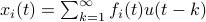 . Then we will impose the bound
  on . In combination with the step size (quantization), this results in
 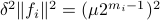 . Let
. Let  be a sequence of i.i.d. sampled random variables from
  . Then we see that
 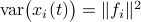 . Hence, one can think of
  as scaling parameter related to the probability with which this dynamic range bound is true.
Next, assume that all the round-off errors are independent and have a variance of  .
Hence, the worst-case variance of computating
.
Hence, the worst-case variance of computating  is
is  . To evaluate the effect of this error on the output, assume for the moment that is identically
  .
Then,
.
Then,  . Similar to , define
  as the component of
  . As before we can compute the variance, this time of the full output signal, which yields
 . Note, these expressions hinge on the indepedence assumption.
Next, define the (infamous) matrices  ,
,  by
by
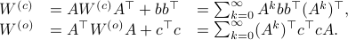
If we assume that the realization is not just minimal, but that  is a controllable pair and that
  is an observable pair, then,
  and
and  .
Now the key observation is that
.
Now the key observation is that 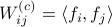 and similarly
 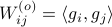 .
Hence, we can write
.
Hence, we can write 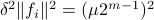 as
as  and indeed
  .
Using these Lyapunov equations we can say goodbye to the infinite-dimensional objects.
.
Using these Lyapunov equations we can say goodbye to the infinite-dimensional objects.
To combine these error terms, let say we have apply a coordinate transformation  , for some .
Specifically, let
, for some .
Specifically, let  be diagonal and defined by
  .
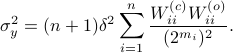
Then one can find that
.
Then one can find that  ,
,  . Where the latter expressions allows to express the output error (variance) by
Now we want to minimize  over all plus some optimal selection of . At this point it looks rather painful. To make it work we first reformulate the problem using the well-known arithmetic-geometric mean inequality
![^{[1]}](eqs/2708305882951756665-130.png) for non-negative sequences
for non-negative sequences ![{a_i}_{iin [n]}](eqs/351138265746961916-130.png) :
:
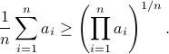
This inequality yields

See that the right term is independent of , hence this is a lower-bound with respect to minimization over . To achieve this (to make the inequality from  an equality), we can select
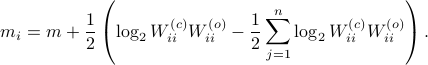
Indeed, as remarked in the paper, is not per se an integer. Nevertheless, by this selection we find the clean expression from to minimize over systems equivalent to , that is, over some transformation matrix . Define a map ![f:mathcal{S}^n_{succ 0}to (0,1]](eqs/6462334851245421111-130.png) by
by
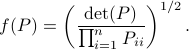
It turns out that  if and only if
  is diagonal. This follows
![^{[2]}](eqs/2708306882823756034-130.png) from Hadamard's inequality.
We can use this map to write
from Hadamard's inequality.
We can use this map to write

Since the term  is invariant under a transformation , we can only optimize over a structural change in realization tuple , that is, we need to make
  and
and  simultaneous diagonal! It turns out that this numerically 'optimal’ realization, denoted
  , is what is called a principal axis realization.
To compute it, diagonalize ,  and define
  . Next, construct the diagonalization
 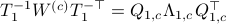 . Then our desired transformation is
  . First, recall that under any the pair
  becomes
  . Plugging in our map yields the transformed matrices
  , which are indeed diagonal.
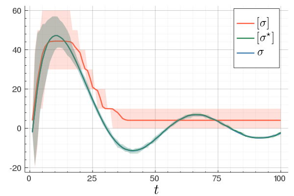 |
At last, we do a numerical test in Julia. Consider a linear system ![A = left[begin{array}{ll} 0.8 & 0.001 0 & -0.5 end{array} right],quad b = left[begin{array}{l} 10 0.1 end{array} right],](eqs/3623138148766993767-130.png)
![c=left[begin{array}{ll} 10 & 0.1 end{array} right],quad d=0.](eqs/42331078943303768-130.png)
To simulate numerical problems, we round the maps |
 and
and  to the closest integer where
 ![[cdot]](eqs/8251583936328055799-130.png) , naive realization
, naive realization ![[sigma]](eqs/4713363484184404481-130.png) and to the optimized one
and to the optimized one ![[sigma^{star}]](eqs/5091401033446485837-130.png) .
We do 100 experiments and show the mean plus the full confidence interval (of the input-output behaviour), the optimized representation is remarkably better.
Numerically we observe that for
.
We do 100 experiments and show the mean plus the full confidence interval (of the input-output behaviour), the optimized representation is remarkably better.
Numerically we observe that for  , which is precisely where the naive
 ![[1]](eqs/8209412804330245758-130.png) : To show this AM-GM inequality, we can use Jensen's inequality for concave functions, that is,
: To show this AM-GM inequality, we can use Jensen's inequality for concave functions, that is, ![mathbf{E}[g(x)]leq g(mathbf{E}[x])](eqs/8492979742681909343-130.png) . We can use the logarithm as our prototypical concave function on
. We can use the logarithm as our prototypical concave function on  and find
  . Then, the result follows.
![[2]](eqs/8209412804333245623-130.png) : The inequality attributed to Hadamard is slightly more difficult to show. In its general form the statement is that
: The inequality attributed to Hadamard is slightly more difficult to show. In its general form the statement is that 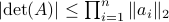 , for
, for  the column of . The inequality becomes an equality when the columns are mutually orthogonal. The intuition is clear if one interprets the determinant as the signed volume spanned by the columns of , which. In case
  , we know that there is
  such that
  , hence, by this simple observation it follows that
Equality holds when the columns are orthogonal, so  must be diagonal, but
  must also hold, hence,
  must be diagonal, and thus must be diagonal, which is the result we use.
A Peculiar Lower Bound to the Spectral Radius |7 March 2020|
tags: math.LA
As a follow up to the previous post, we discuss a lower bound, given as exercise P7.1.14 in (GvL13).
I have never seen this bound before, especially not with the corresponding proof, so here we go.
Given any , we have the following lower bound:
which can be thought of as a sharpening of the bound 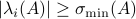 .
In the case of a singular , the bound is trivial
.
In the case of a singular , the bound is trivial  , but in the general setting it is less obvious.
To prove that this holds we need a few ingredients. First, we need that for any
, but in the general setting it is less obvious.
To prove that this holds we need a few ingredients. First, we need that for any  we have
  .
Then, we construct two decompositions of , (1) the Jordan Normal form
.
Then, we construct two decompositions of , (1) the Jordan Normal form  , and (2) the Singular Value Decomposition
  .
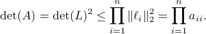
Using the multiplicative property of the determinant, we find that
.
Using the multiplicative property of the determinant, we find that
Hence, since 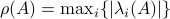 it follows that
 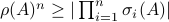 and thus we have the desired result.
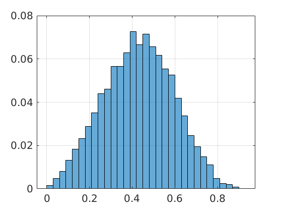 |
(Update 8 March) It is of course interesting to get insight in how sharp this bound is, in general. To that end we consider random matrices |
 with
with 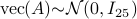 . When we compute the relative error
  for
for  samples we obtain the histogram as shown on the left. Clearly, the relative error is not concentrated near
 (GvL13) G.H. Golub and C.F. Van Loan: ‘‘Matrix Computations’’, 2013 John Hopkins University Press.
Spectral Radius vs Spectral Norm |28 Febr. 2020|
tags: math.LA, math.DS
Lately, linear discrete-time control theory has start to appear in areas far beyond the ordinary. As a byproduct, papers start to surface which claim that stability of linear discrete-time systems

is characterized by  .
The confunsion is complete by calling this object the spectral norm of a matrix .
Indeed, stability of is not characterized by
.
The confunsion is complete by calling this object the spectral norm of a matrix .
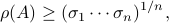
Indeed, stability of is not characterized by  , but by
 ![rho(A):=max_{iin [n]}|lambda_i(A)|](eqs/8716262940618826552-130.png) .
If , then all absolute eigenvalues of are strictly smaller than one, and hence for
.
If , then all absolute eigenvalues of are strictly smaller than one, and hence for  ,
,  .
This follows from the Jordan form of in combination with the simple observation that for
.
This follows from the Jordan form of in combination with the simple observation that for  ,
,  .
.
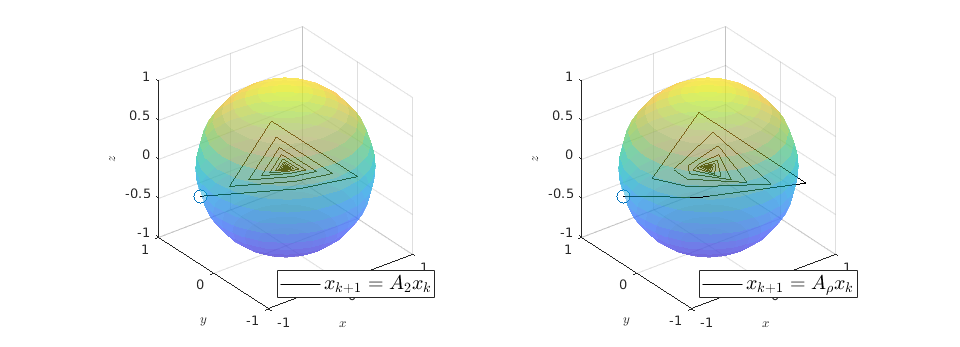
To continue, define two sets;  and
and  .
Since
.
Since  we have
  . Now, the main question is, how much do we lose by approximating
  with
with  ? Motivation to do so is given by the fact that
  is a norm and hence a convex function, i.e., when given a convex polytope
  with vertices
  , if
, if  , then
  . Note that
  is not a norm, can be without
  (consider an upper-triangular matrix with zeros on the main diagonal), the triangle inequality can easily fail as well. For example, let
![A_1 = left[begin{array}{ll} 0 & 1 0 & 0 end{array}right], quad A_2 = left[begin{array}{ll} 0 & 0 1 & 0 end{array}right],](eqs/6730715665771009175-130.png)
Then  , but
, but  , hence
  fails to hold.
A setting where the aforementioned property of might help is Robust Control, say we want to assess if some algorithm rendered a compact convex set
fails to hold.
A setting where the aforementioned property of might help is Robust Control, say we want to assess if some algorithm rendered a compact convex set  , filled with 's, stable.
As highlighted before, we could just check if all extreme points of are members of
, filled with 's, stable.
As highlighted before, we could just check if all extreme points of are members of  , which might be a small and finite set.
Thus, computationally, it appears to be attractive to consider over the generic .
, which might be a small and finite set.
Thus, computationally, it appears to be attractive to consider over the generic .
As a form of critique, one might say that is a lot larger than .
Towards such an argument, one might recall that  . Indeed,
  if
if![^{[3]}](eqs/2708307882947756447-130.png)
 , but
, but  . Therefore, it seems like the set of for which considering over
  is reasonable, is negligibly small.
To say a bit more, since
is reasonable, is negligibly small.
To say a bit more, since![^{[4]}](eqs/2708308882819756064-130.png)
 we see that we can always find a ball with non-zero volume fully contained in .
Hence, is at least locally dense in
we see that we can always find a ball with non-zero volume fully contained in .
Hence, is at least locally dense in  . The same holds for
  (which is more obvious).
So in principle we could try to investigate
(which is more obvious).
So in principle we could try to investigate  . For
. For  , the sets agree, which degrades asymptotically.
However, is this the way to go? Lets say we consider the set
, the sets agree, which degrades asymptotically.
However, is this the way to go? Lets say we consider the set  . Clearly, the sets
  and are different, even in volume, but for sufficiently large
  , should we care? The behaviour they parametrize is effectively the same.
We will stress that by approximating  with , regardless of their volumetric difference, we are ignoring a full class of systems and miss out on a non-neglible set of behaviours.
To see this, any system described by is contractive in the sense that
with , regardless of their volumetric difference, we are ignoring a full class of systems and miss out on a non-neglible set of behaviours.
To see this, any system described by is contractive in the sense that  , while systems in are merely asymptotically stable. They might wander of before they return, i.e., there is no reason why for all
  we must have
  . We can do a quick example, consider the matrices
![A_2 = left[begin{array}{lll} 0 & -0.9 & 0.1 0.9 & 0 & 0 0 & 0 & -0.9 end{array}right], quad A_{rho} = left[begin{array}{lll} 0.1 & -0.9 & 1 0.9 & 0 & 0 0 & 0 & -0.9 end{array}right].](eqs/7939256391259616851-130.png)
Then  ,
,  and both
  and
and  have
have  .
We observe that indeed is contractive, for any initial condition on
.
We observe that indeed is contractive, for any initial condition on  , we move strictly inside the sphere, whereas for , when starting from the same initial condition, we take a detour outside of the sphere before converging to . So although and have the same spectrum, they parametrize different systems.
 |
In our deterministic setting this would mean that we would confine our statespace to a (solid) sphere with radius  , instead of .
Moreover, in linear optimal control, the resulting closed-loop system is usually not contractive.
Think of the infamous pendulum on a cart. Being energy efficient has usually nothing to do with taking the shortest, in the Euclidean sense, path.
, instead of .
Moreover, in linear optimal control, the resulting closed-loop system is usually not contractive.
Think of the infamous pendulum on a cart. Being energy efficient has usually nothing to do with taking the shortest, in the Euclidean sense, path.
: Recall, 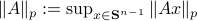 . Then, let
  be some eigenvector of . Now we have
  . Since this eigenvalue is arbitrary it follows that
  .
.
: Let 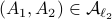 then
then  . This follows from the being a norm.
![[3]](eqs/8209412804332245752-130.png) : Clearly, if , we have
: Clearly, if , we have  . Now, when
  , does this imply that ? The answer is no, consider
![A' = left[begin{array}{lll} 0.9 & 0 & 0 0 & 0.1 & 0 0 & 0.1 & 0.1 end{array}right].](eqs/1479234184051328788-130.png)
Then,  , yet,
  . For the full set of conditions on such that see this paper by Goldberg and Zwas.
![[4]](eqs/8209412804335245617-130.png) : Recall that
: Recall that  . This expression is clearly larger or equal to
  .
.
A Special Group, Volume Preserving Feedback |16 Nov. 2019|
tags: math.LA, math.DS
This short note is inspired by the beautiful visualization techniques from Duistermaat and Kolk (DK1999).
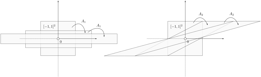
Let's say we have a -dimensional linear discrete-time dynamical system , which preserves the volume of the cube ![[-1,1]^2](eqs/7220646983027292775-130.png) under the dynamics, i.e.
under the dynamics, i.e. ![mathrm{Vol}([-1,1]^2)=mathrm{Vol}(A^k[-1,1]^2)](eqs/6078350520623442645-130.png) for any
for any  .
.
Formally put, this means that is part of a certain group, specifically, consider some field  and
define the Special Linear group by
and
define the Special Linear group by

Now, assume that we are only interested in matrices  such that the cube remains bounded under the dynamics, i.e.,
 ![lim_{kto infty}A^k[-1,1]^2](eqs/6180125548835686349-130.png) is bounded. In this scenario we restrict our attention to
is bounded. In this scenario we restrict our attention to  . To see why this is needed, consider
  and both with determinant
  :
:
![A_1 = left[ begin{array}{ll} 2 & 0 0 & frac{1}{2} end{array}right], quad A_2 = left[ begin{array}{ll} 1 & 2 0 & 1 end{array}right],](eqs/4004660008936570769-130.png)
If we look at the image of under both these maps (for several iterations), we see that volume is preserved, but also clearly that the set is extending indefinitely in the horizontal direction.
 |
To have a somewhat interesting problem, assume we are given  with
with  while it is our task to find a
  such that
  , hence, find feedback which not only preserves the volume, but keeps any set of initial conditions (say ) bounded over time.
Towards a solution, we might ask, given any what is the nearest (in some norm) rotation matrix? This turns out to be a classic question, starting from orthogonal matrices, the solution to  is given by
  , where
  follows from the SVD of , .
Differently put, when we use a polar decomposition of ,
follows from the SVD of , .
Differently put, when we use a polar decomposition of ,  , then the solution is given by
  . See this note for a quick multiplier proof.
An interesting sidenote, problem is well-defined since
. See this note for a quick multiplier proof.
An interesting sidenote, problem is well-defined since  is compact. To see this, recall that for any
  we have
  , hence the set is bounded, plus is the pre-image of
  under
under  ,
,  , hence the set is closed as well.
This is great, however, we would like to optimize over  instead. To do so, one usually resorts to simply checking the sign - and if necessary - flipping it via finding the closest matrix with a change in determinant sign.
We will see that by selecting appropriate coordinates we can find the solution without this checking of signs.
instead. To do so, one usually resorts to simply checking the sign - and if necessary - flipping it via finding the closest matrix with a change in determinant sign.
We will see that by selecting appropriate coordinates we can find the solution without this checking of signs.
For today we look at  and largely follow (DK1999), for such a -dimensional matrix, the determinant requirement translates to
  . Under the following (invertible) linear change of coordinates
![left[ begin{array}{l} a d b c end{array}right] = left[ begin{array}{llll} 1 & 1 & 0 & 0 1 & -1 & 0 & 0 0 & 0 & 1 & 1 0 & 0 & 1 & -1 end{array}right] left[ begin{array}{l} p q r s end{array}right]](eqs/6118233270205082065-130.png)
 becomes
  , i.e., for any pair
  the point
  runs over a circle with radius
  . Hence, we obtain the diffeomorphism
 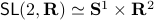 . We can use however a more pretty diffeomorphism of the sphere and an open set in
  . To that end, use the diffeomorphism:
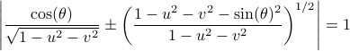
![(theta,(u,v)) mapsto frac{1}{sqrt{1-u^2-v^2}} left[ begin{array}{ll} cos(theta)+u & -sin(theta)+v sin(theta)+v & cos(theta)-u end{array}right] in mathsf{SL}(2,mathbf{R}),](eqs/6656969251929689946-130.png)
for  (formal way of declaring that
  should not be any real number) and the pair
  being part of
  (the open unit-disk).
To see this, recall that the determinant is not a linear operator.
Since we have a -dimensional example we can explicitly compute the eigenvalues of any (plug into the characteristic equation) and obtain:
(the open unit-disk).
To see this, recall that the determinant is not a linear operator.
Since we have a -dimensional example we can explicitly compute the eigenvalues of any (plug into the characteristic equation) and obtain:
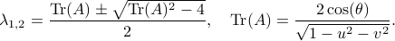
At this point, the only demand on the eigenvalues is that  . Therefore, when we would consider within the context of a discrete linear dynamical system , is either a saddle-point, or we speak of a marginally stable system (
 ).
We can visualize the set of all marginally stable , called
).
We can visualize the set of all marginally stable , called  , defined by all
 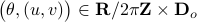 satisfying
(DK1999) J.J. Duistermaat and J.A.C. Kolk : ‘‘Lie Groups’’, 1999 Springer.
Simple Flow Algorithm to Compute the Operator Norm |4 Nov. 2019|
tags: math.LA
Using the ideas from the previous post, we immediately obtain a dynamical system to compute  for any
  (symmetric positive definite matrices).
Here we use the vector field
(symmetric positive definite matrices).
Here we use the vector field  , defined by
  and denote a solution by
  , where
  is the initial condition. Moreover, define a map
  by
by  . Then
 , where
  is the eigenvector corresponding to the largest eigenvalue.
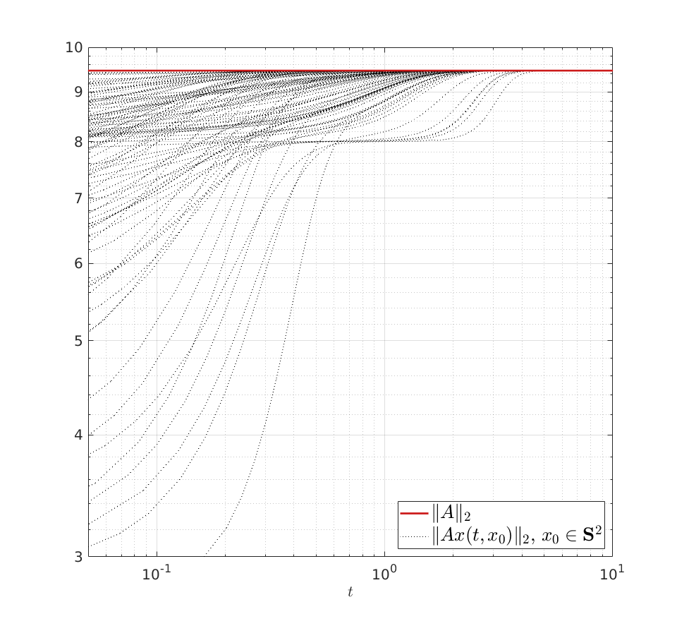 |
We can do a simple example, let ![A = left[ begin{array}{lll} 8 & 2 & 0 2 & 4 & 2 0 & 2 & 8 end{array}right]](eqs/3487469526425297871-130.png)
with |
 . Indeed, when given 100
  , we observe convergence. To apply this in practice we obviously need to discretize the flow. To add to that, if we consider the discrete-time version of
  ,
,  we can get something of the form
  , which is indeed the
 Finite Calls to Stability | 31 Oct. 2019 |
tags: math.LA, math.DS
Consider an unknown dynamical system parametrized by  .
In this short note we look at a relatively simple, yet neat method to assess stability of via finite calls to a particular oracle. Here, we will follow the notes by Roman Vershynin (RV2011).
.
In this short note we look at a relatively simple, yet neat method to assess stability of via finite calls to a particular oracle. Here, we will follow the notes by Roman Vershynin (RV2011).
Assume we have no knowledge of , but we are able to obtain  for any desired
  . It turns out that we can use this oracle to bound from above.
First, recall that since is symmetric,  . Now, the common definition of is
  . The constraint set
  is not per se convenient from a computational point of view. Instead, we can look at a compact constraint set:
 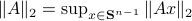 , where
  is the sphere in .
The latter formulation has an advantage, we can discretize these compact constraints sets and tame functions over the individual chunks.
is the sphere in .
The latter formulation has an advantage, we can discretize these compact constraints sets and tame functions over the individual chunks.
To do this formally, we can use  -nets, which are convenient in quantitative analysis on compact metric spaces
  . Let
. Let  be a -net for
  if
if  . Hence, we measure the amount of balls to cover .
For example, take  as our metric space where we want to bound
  (the cardinality, i.e., the amount of balls). Then, to construct a minimal set of balls, consider an -net of balls
  , with
  . Now the insight is simply that
  .
Luckily, we understand the volume of -dimensional Euclidean balls well such that we can establish
.
Luckily, we understand the volume of -dimensional Euclidean balls well such that we can establish

Which is indeed sharper than the bound from Lemma 5.2 in (RV2011).
Next, we recite Lemma 5.4 from (RV2011). Given an -net for with  we have
This can be shown using the Cauchy-Schwartz inequality. Now, it would be interesting to see how sharp this bound is.
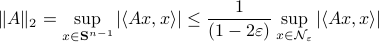
To that end, we do a -dimensional example ( ). Note, here we can easily find an optimal grid using polar coordinates. Let the unknown system be parametrized by
![A = left[ begin{array}{ll} 0.1 & -0.75 -0.75 & 0.1 end{array}right]](eqs/8870555444473195760-130.png)
such that  . In the figures below we compute the upper-bound to for several nets
  .
Indeed, for finer nets, we see the upper-bound approaching
.
Indeed, for finer nets, we see the upper-bound approaching  . However, we see that the convergence is slow while being inversely related to the exponential growth in .
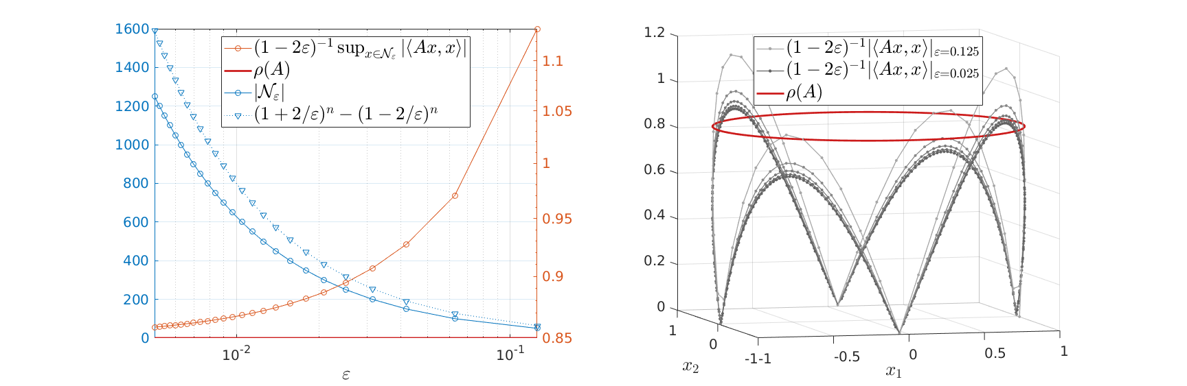 |
Overall, we see that after about a 100 calls to our oracle we can be sure about being exponentially stable.
Here we just highlighted an example from (RV2011), at a later moment we will discuss its use in probability theory.
Help the (skinny) Hedgehogs | 31 Oct. 2019 |
tags: math.LA, other.Nature
In this first post we will see that the ‘‘almost surely’’ in the title is not only hinting at stochasticity.
For a long time this picture - as taken from Gabriel Peyré his outstanding twitter feed - has been on a wall in our local wildlife (inc. hedgehogs) shelter. This has lead to a few fun discussions and here we try to explain the picture a bit more.
Let  . Now, we want to find the largest ball
  within
  . We can find that
  is given by
  with
with  . This follows the most easily from geometric intuition.
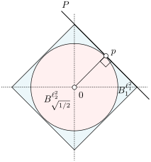 |
To prove it, see that |
 ‘‘similar’’ faces, without loss of generality we take the one in the positive orthant of
  -dimensional plane
  the closest (in
  for
for  and
and  . Thus the normal (direction) is given by
  . To find
  , observe that for
  we have
  . Hence we have
  . Now, let
  and define the other
  for any
  . The inscribed ball shrinks to
 Besides being a fun visualization of concentration, this picture means a bit more to me. For years I have been working at the Wildlife shelter in Delft and the moment has come where the lack of financial support from surrounding municipalities is becoming critical. As usual, this problem can be largely attributed to bureaucracy and the exorbitant amount of managers this world has. Nevertheless, the team in Delft and their colleagues around the country do a fantastic job in spreading the word (see Volkskrant, RTLnieuws). Lets hope Delft, and it neighbours, finally see value in protecting the local wildlife we still have.