Posts (10) containing the 'math.OC’ (Optimization and Control) tag:
Communities |July 02, 2024|
tags: math.OC
As the thesis is printed, it is time to reflect.
Roughly 1 year ago I got the wonderful advice from Roy Smith that whatever you do, you should be part of a community. This stayed with me as four years ago I wrote on my NCCR Automation profile page that “Control problems of the future cannot be solved alone, you need to work together.” and I finally realized — may it be in retrospect — what this really means, I was being kindly welcomed to several communities.
Just last week at the European Control Conference (ECC24), Angela Fontan and Matin Jafarian organized a lunch session on peer review in our community and as Antonella Ferrara emphasized throughout, you engage in the process to contribute to the community, your community. As such, a high quality — and sustainable — conference is intimately connected to the feeling of community. Especially since the conference itself feeds back into our feeling of community (as I am sure you know, everything is just feedback loops..).
ECC24 was a fantastic example when it comes to strengthening that feeling of community and other examples that come to mind are the inControl podcast by Alberto Padoan, Autonomy Talks by Gioele Zardini, the IEEE CSS magazine, the IEEE CSS road map 2030 and recently, the KTH reading group on Control Theory: Twenty-Five Seminal Papers (1932-1981) organized by Miguel Aguiar. The historical components are important not only to better understand our community (the why, how and what), but to always remember we build upon our predecessors, we are part of the same community. Of course, the NCCR Automation contributed enormously and far beyond Switzerland (fellowships, symposia, workshops, …), but even closer to home, ever since the previous century, the Dutch Institute of Systems and Control (DISC) has done a remarkable job bringing and keeping all researchers and students together (MSc programs, a national graduate school, Benelux meetings, …).
The importance of community is sometimes linked to being in need of recognition and to working more effective when in competition. I am sure this is true for some and I am even more sure this is enforced in fields where research is expensive and funding is scarce. Yet, that vast majority of members of the scientific community are not PIs, but students, and for us the community is critically important to create and enforce a sense of belonging. The importance of belonging are widely known — not only in the scientific community — and most of the problems we have here on earth can be directly linked to a lack of belonging and community (as beautifully formulated in Pale Blue Dot by Carl Sagan).
Celebrating personal successes is of great importance, we need our heros, but I want to be part of a scientific community where we focus on progress of the community, what did we solve, what are our open problems, and how do we go about solving them? Looking back, I happy to see it seems I am. Thank you!
Weekend read |May 14, 2023|
tags: math.OC
The ‘‘Control for Societal-scale Challenges: Road Map 2030’’ by the IEEE Control Systems Society (Eds. A. M. Annaswamy, K. H. Johansson, and G. J. Pappas) was published a week ago. This roadmap is a remarkable piece of work, over 250 pages, an outstanding list of authors and coverage of almost anything you can imagine, and more.
If you somehow found your way to this website, then I can only strongly recommend reading this document. Despite many of us being grounded in traditional engineering disciplines, I do agree with the sentiment of this roadmap that the most exciting (future) work is interdisciplinary, this is substantiated by many examples from biology. Better yet, it is stressed that besides familiarizing yourself with the foundations, it is of quintessential importance (and fun I would say) to properly dive into the field where you hope to apply these tools.
‘‘Just because you can formulate and solve an optimization problem does not mean that you have the correct or best cost function.’’ p. 32
Section 4.A on Learning and Data-Driven Control also contains many nice pointers, sometimes alluding to a slight disconnect between practice and theory.
‘‘Sample complexity may only be a coarse measure in this regard, since it is not just the number of samples but the “quality” of the samples that matters.’’ p. 142
The section on safety is also inspiring, just stability will not be enough anymore. However, the most exciting part for me was Chapter 6 on education. The simple goal of making students excited early-on is just great. Also, the aspiration to design the best possible material as a community is more than admirable.
Standing on the shoulders of giants |April 3, 2023|
tags: math.OC
One of the most illuminating activities one can undertake is to go back in time and see how the giants in (y)our field shaped the present. Sadly, several of our giants passed away recently and I want to highlight one of them in particular: Roger W. Brockett.
It is very rare to find elegant and powerful theories in sytems and control that are not related to Brockett somehow, better yet, many powerful theories emerged directly from his work. Let me highlight five topics/directions I find remarkably beautiful:
(Lie algebras): As put by Brockett himself, it is only natural to study the link between Lie theory and control theory since the two are intimately connected through differential equations |1.2|. ‘‘Completing this triangle’’ turned out to be rather fruitful, in particular via Frobenius’ theorem. Brockett played a key role in bringing Lie theoretic methods to control theory, a nice example is his 1973 paper on control systems on spheres (in general, his work on bilinear systems was of great interest) |5|.
(Differential geometric methods): Together with several others, Brockett was one of the first to see how differential geometric methods allowed for elegantly extending ideas from linear control (linear algebra) to the realm of nonlinear control. A key event is the 1972 conference co-organized with David Mayne |1|. See also |2| for a short note on the history of geometric nonlinear control written by Brockett himself.
(Brockett's condition): After pioneering work on (local) nonlinear controllability in the 70s it was observed (by means of low-dimensional counterexamples) that controllability is not sufficient for the existence of a stabilizing continuous feedback. This observation was firmly established in the (1982) 1983 paper by Brockett |3| where he provides his topological necessary condition (Theorem 1 (iii)) for the existence of a stabilizing differentiable feedback, i.e.
 must be locally onto (the same is true for continuous feedback). Formally speaking, this paper is not the first (see Geometrical Methods of Nonlinear Analysis and this paper by Zabczyk), yet, this paper revolutionized how to study necessary conditions for nonlinear stabilization and inspired an incredible amount of work.
(Nonlinear control systems): Although we are still far from the definitive control system (modelling) framework, Brockett largely contributed to a better understanding of structure. Evidently, this neatly intertwines with the previous points on bilinear systems (Lie algebras) and differential geometry, however, let me also mention that the fiber bundle perspective (going beyond Cartesian products) is often attributed to Brockett |4|.
(Dynamical systems perspective on optimization): We see nowadays still more and more work on the continuous-time (and system theoretic) viewpoint with respect to optimization algorithms. One can argue that Brockett was also of great importance here. It is not particularly surprising that one can study gradient flows to better understand gradient descent algorithms, however, it turned out that one can understand a fair amount of routines from (numerical) linear algebra through the lens of (continuous-time) dynamical systems. Brockett initiated a significant part of this work with his 1988 paper on the applications of the double bracket equation
![dot{H}=[H,[H,N]]](eqs/229228239358215717-130.png) |6|. For a more complete overview, including a foreword by Brockett, see Optimization and Dynamical Systems.
|6|. For a more complete overview, including a foreword by Brockett, see Optimization and Dynamical Systems.
References (all by Brockett).
|1|: Geometric Methods in System Theory - Proceedings of the NATO Advanced Study Institute held at London, England, August 27-Septernber 7, 1973, ed. with Mayne, D. Reidel Publishing Company (1973).
|1.2|: Chapter: Lie Algebras and Lie groups in Control Theory in |1|.
|2|: The early days of geometric nonlinear control, Automatica (2014).
|3|: Asymptotic stability and feedback stabilization, Differential Geometric Control Theory, ed. with Millman and Sussmann, Birkhäuser (1983).
|4|: Control theory and analytical mechanics, Geometric Control Theory, Lie Groups: History,
Frontiers and Applications, Vol. VII, ed. Martin and Hermann, Math Sci Press, (1976).
|5|: Lie Theory and Control Systems Defined on Spheres, SIAM Journal on Applied Mathematics (1973).
|6|: Dynamical systems that sort lists and solve linear programming problems, IEEE CDC (1988).
See also this 2022 interview (video) with John Baillieul and the foreword to this book for more on the person behind the researcher.
Co-observability |6 January 2022|
tags: math.OC
A while ago Prof. Jan H. van Schuppen published his book Control and System Theory of Discrete-Time Stochastic Systems. In this post I would like to highlight one particular concept from the book: (stochastic) co-observability, which is otherwise rarely discussed.
We start with recalling observability. Given a linear-time-invariant system with  ,
,  :
:
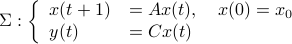
one might wonder if the initial state  can be recovered from a sequence of outputs
  . (This is of great use in feedback problems.) By observing that
  ,
,  ,
,  one is drawn to the observability matrix
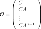
Without going into detectability, when  is full-rank, one can (uniquely) recover (proof by contradiction). If this is the case, we say that
  , or equivalenty the pair
  , is observable. Note that using a larger matrix (more data) is redudant by the Cayley-Hamilton theorem (If would not be full-rank, but by adding
  “from below” it would somehow be full-rank, one would contradict the Cayley-Hamilton theorem.).
Also note that in practice one does not “invert” but rather uses a (Luenberger) observer (or a Kalman filter).
“from below” it would somehow be full-rank, one would contradict the Cayley-Hamilton theorem.).
Also note that in practice one does not “invert” but rather uses a (Luenberger) observer (or a Kalman filter).
Now lets continue with a stochastic (Gaussian) system, can we do something similar? Here it will be even more important to only think about observability matrices as merely tools to assert observability. Let  be a zero-mean Gaussian random variable with covariance
  and define for some matrices
  and
and  the stochastic system
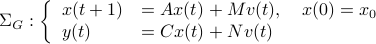
We will assume that  is asymptotically (exponentially stable) such that the Lyapunov equation describing the (invariant) state-covariance is defined:
Now the support of the state  is the range of
  .
.
A convenient tool to analyze  will be the characteristic function of a Gaussian random variable
  , defined as
 ![varphi(omega)=mathbf{E}[mathrm{exp}(ilangle omega, Xrangle)]](eqs/1509536698066778096-130.png) .
It can be shown that for a Gaussian random variable
.
It can be shown that for a Gaussian random variable 
 .
With this notation fixed, we say that
.
With this notation fixed, we say that  is stochastically observable on the internal
  if the map
![x(t)mapsto mathbf{E}[mathrm{exp}(ilangle omega,bar{y}rangle|mathcal{F}^{x(t)}],quad bar{y}=(y(t),dots,y(t+k))in mathbf{R}^{pcdot(k+1)}quad forall omega](eqs/853891715523836887-130.png)
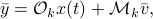
is injective on the support of (note the  ). The intuition is the same as before, but now we want the state to give rise to an unique (conditional) distribution. At this point is seems rather complicated, but as it turns out, the conditions will be similar to ones from before. We start by writing down explicit expressions for
  , as
, as
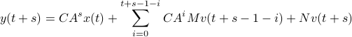
we find that
for  the observability matrix corresponding to the data (length) of ,
  a matrix containing all the noise related terms and
  a stacked vector of noises similar to . It follows that
 ![x(t)mapsto mathbf{E}[mathrm{exp}(ilangle omega,bar{y})|mathcal{F}^{x(t)}]](eqs/1452358234763943133-130.png) is given by
is given by  , for
, for ![mathcal{Q}_k = mathbf{E}[mathcal{M}_kbar{v}bar{v}^{mathsf{T}}mathcal{M}_k^{mathsf{T}}]](eqs/8712945555052273745-130.png) . Injectivity of this map clearly relates directly to injectivity of
. Injectivity of this map clearly relates directly to injectivity of 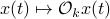 . As such (taking the support into account), a neat characterization of stochastic observability is that
 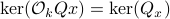 .
.
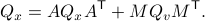
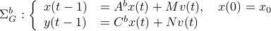
Then, to introduce the notion of stochastic co-observability we need to introduce the backward representation of a system. We term system representations like and “forward” representations as  . Assume that
  , then see that the forward representation of a system matrix, denoted
  is given by
 ![A^f = mathbf{E}[x(t+1)x(t)^{mathsf{T}}]Q_x^{-1}](eqs/3247376240463532393-130.png) . In a similar vein, the backward representation is given by
. In a similar vein, the backward representation is given by ![A^b=mathbf{E}[x(t-1)x(t)^{mathsf{T}}]Q_x^{-1}](eqs/3587697042984921977-130.png) .
Doing the same for the output matrix
.
Doing the same for the output matrix  yields
 ![C^b=mathbf{E}[y(t-1)x(t)^{mathsf{T}}]Q_x^{-1}](eqs/2184503885116254462-130.png) and thereby the complete backward system
and thereby the complete backward system
Note, to keep and fixed, we adjust the distribution of  .
Indeed, when is not full-rank, the translation between forward and backward representations is not well-defined. Initial conditions
.
Indeed, when is not full-rank, the translation between forward and backward representations is not well-defined. Initial conditions  cannot be recovered.
To introduce co-observability, ignore the noise for the moment and observe that  ,
,  , and so forth.
We see that when looking at observability using the backward representation, we can ask if it possible to recover the current state using past outputs. Standard observability looks at past states instead. With this in mind we can define stochastic co-observability on the interval
, and so forth.
We see that when looking at observability using the backward representation, we can ask if it possible to recover the current state using past outputs. Standard observability looks at past states instead. With this in mind we can define stochastic co-observability on the interval  be demanding that the map
![x(t)mapsto mathbf{E}[mathrm{exp}(ilangle omega,bar{y}^brangle|mathcal{F}^{x(t)}],quad bar{y}^b=(y(t-1),dots,y(t-k-1))in mathbf{R}^{pcdot(k+1)}quad forall omega](eqs/2807210638750947645-130.png)
is injective on the support of (note the ). Of course, one needs to make sure that  is defined. It is no surprise that the conditions for stochastic co-observability will also be similar, but now using the co-observability matrix. What is however remarkable, is that these notions do not always coincide.
Lets look at when this can happen and what this implies. One reason to study these kind of questions is to say something about (minimal) realizations of stochastic processes. Simply put, what is the smallest (as measured by the dimension of the state ) system that gives rise to a certain output process. When observability and co-observability do not agree, this indicates that the representation is not minimal. To get some intuition, we can do an example as adapted from the book. Consider the scalar (forward) Gaussian system

for  . The system is stochastically observable as
  and
and  . Now for stochastic co-observability we see that
 ![c^b=mathbf{E}[y(t-1)x(t)]q_x^{-1}]=0](eqs/6755659394537019237-130.png) , as such the system is not co-observable. What this shows is that
, as such the system is not co-observable. What this shows is that  behaves as a Gaussian random variable, no internal dynamics are at play and such a minimal realization is of dimension
  .
.
For this and a lot more, have a look at the book!
Fair convex partitioning |26 September 2021|
tags: math.OC
When learning about convex sets, the definitions seem so clean that perhaps you think all is known what could be known about finite-dimensional convex geometry. In this short note we will look at a problem which is still largely open beyond the planar case. This problem is called the fair partitioning problem.
In the  -dimensional case, the question is the following, given any integer
  , can a convex set
  be divided into convex sets all of equal area and perimeter.
Differently put, does there exist a fair convex partitioning, see Figure 1.
be divided into convex sets all of equal area and perimeter.
Differently put, does there exist a fair convex partitioning, see Figure 1.
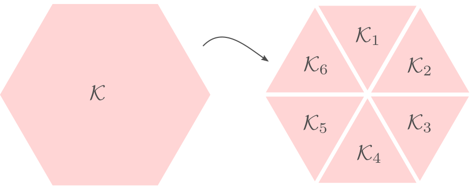 |
Figure 1:
A partition of |
 fair convex sets.
This problem was affirmatively solved in 2018, see this paper.
As you can see, this work was updated just a few months ago. The general proof is involved, lets see if we can do the case for a compact set and  .
.
First of all, when splitting  (into just two sets) you might think of many different methods to do so. What happens when the line is curved? The answer is that when the line is curved, one of the resulting sets must be non-convex, compare the options in Figure 2.
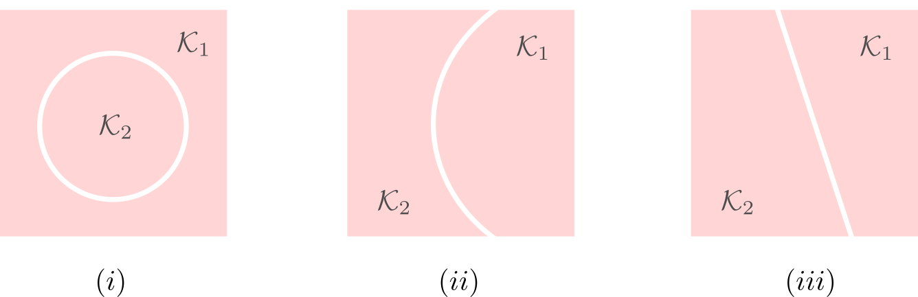 |
Figure 2:
A partitioning of the square in |
 into two convex sets can only be done via a straight cut.
This observation is particularly useful as it implies we only need to look at two points on the boundary of (and the line between them). As is compact we can always select a cut such that the resulting perimeters of  and
and  are equal.
Let us assume that the points  and
and  in Figure 3.(i) are like that. If we start moving them around with equal speed, the resulting perimeters remain fixed. Better yet, as the cut is a straight-line, the volumes (area) of the resulting set and change continuously. Now the result follows from the Intermediate Value Theorem and seeing that we can flip the meaning of and , see Figure 3.(iii).
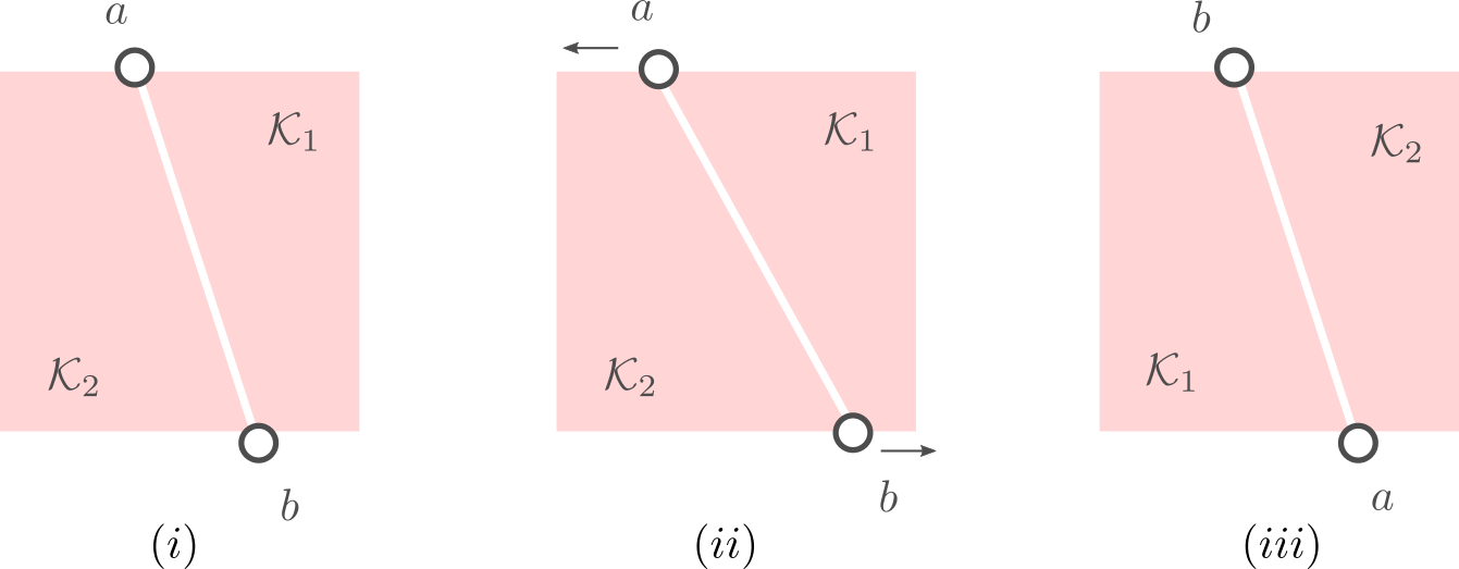 |
Figure 3:
By moving the points |
Solving Linear Programs via Isospectral flows |05 September 2021|
tags: math.OC, math.DS, math.DG
In this post we will look at one of the many remarkable findings by Roger W. Brockett. Consider a Linear Program (LP)

parametrized by the compact set 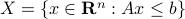 and a suitable triple
  .
As a solution to
.
As a solution to  can always be found to be a vertex of , a smooth method to solve seems somewhat awkward.
We will see that one can construct a so-called isospectral flow that does the job.
Here we will follow Dynamical systems that sort lists, diagonalize matrices and solve linear programming problems, by Roger. W. Brockett (CDC 1988) and the book Optimization and Dynamical Systems edited by Uwe Helmke and John B. Moore (Springer 2ed. 1996).
Let have
can always be found to be a vertex of , a smooth method to solve seems somewhat awkward.
We will see that one can construct a so-called isospectral flow that does the job.
Here we will follow Dynamical systems that sort lists, diagonalize matrices and solve linear programming problems, by Roger. W. Brockett (CDC 1988) and the book Optimization and Dynamical Systems edited by Uwe Helmke and John B. Moore (Springer 2ed. 1996).
Let have  vertices, then one can always find a map
 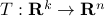 , mapping the simplex
  onto .
Indeed, with some abuse of notation, let
onto .
Indeed, with some abuse of notation, let  be a matrix defined as
  , for
, for  , the vertices of .
Before we continue, we need to establish some differential geometric results. Given the Special Orthogonal group  , the tangent space is given by
  . Note, this is the explicit formulation, which is indeed equivalent to shifting the corresponding Lie Algebra.
The easiest way to compute this is to look at the kernel of the map defining the underlying manifold.
. Note, this is the explicit formulation, which is indeed equivalent to shifting the corresponding Lie Algebra.
The easiest way to compute this is to look at the kernel of the map defining the underlying manifold.
Now, following Brockett, consider the function  defined by
  for some
  . This approach is not needed for the full construction, but it allows for more intuition and more computations.
To construct the corresponding gradient flow, recall that the (Riemannian) gradient at
. This approach is not needed for the full construction, but it allows for more intuition and more computations.
To construct the corresponding gradient flow, recall that the (Riemannian) gradient at  is defined via
 ![df(Theta)[V]=langle mathrm{grad},f(Theta), Vrangle_{Theta}](eqs/666734593389601294-130.png) for all
for all  . Using the explicit tangent space representation, we know that
  with
with  .
Then, see that by using
.
Then, see that by using

we obtain the gradient via
![df(Theta)[V]=lim_{tdownarrow 0}frac{f(Theta+tV)-f(Theta)}{t} = langle QTheta N, Theta Omega rangle - langle Theta N Theta^{mathsf{T}} Q Theta, Theta Omega rangle.](eqs/2651725126600601485-130.png)
This means that (the minus is missing in the paper) the (a) gradient flow becomes

Consider the standard commutator bracket ![[A,B]=AB-BA](eqs/2726051070798907854-130.png) and see that for
and see that for  one obtains from the equation above (typo in the paper)
![dot{H}(t) = [H(t),[H(t),N]],quad H(0)=Theta^{mathsf{T}}QThetaquad (2).](eqs/8308117426617579905-130.png)
Hence,  can be seen as a reparametrization of a gradient flow.
It turns out that has a variety of remarkable properties. First of all, see that
can be seen as a reparametrization of a gradient flow.
It turns out that has a variety of remarkable properties. First of all, see that  preserves the eigenvalues of
  .
Also, observe the relation between extremizing
.
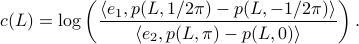
Also, observe the relation between extremizing  and the function
  defined via
  . The idea to handle LPs is now that the limiting will relate to putting weight one the correct vertex to get the optimizer, gives you this weight as it will contain the corresponding largest costs.
In fact, the matrix  can be seen as an element of the set
  .
This set is in fact a
.
This set is in fact a  -smooth compact manifold as it can be written as the orbit space corresponding to the group action
  ,
,
 , one can check that this map satisfies the group properties. Hence, to extremize over
  , it appears to be appealing to look at Riemannian optimization tools indeed. When doing so, it is convenient to understand the tangent space of
  . Consider the map defining the manifold
  ,
,  . Then by the construction of
  , see that
 ![dh(Theta)[V]=0](eqs/8898228761859333701-130.png) yields the relation
yields the relation ![[H,Omega]=0](eqs/197549272010137556-130.png) for any
for any  .
.
For the moment, let  such that
  and
and  .
First we consider the convergence of .
Let have only distinct eigenvalues, then
.
First we consider the convergence of .
Let have only distinct eigenvalues, then  exists and is diagonal.
Using the objective from before, consider
exists and is diagonal.
Using the objective from before, consider  and see that by using the skew-symmetry one recovers the following
![begin{array}{lll} frac{d}{dt}mathrm{Tr}(H(t)N) &=& mathrm{Tr}(N [H,[H,N]]) &=& -mathrm{Tr}((HN-NH)^2) &=& |HN-NH|_F^2. end{array}](eqs/6018522323896655448-130.png)
This means the cost monotonically increases, but by compactness converges to some point  . By construction, this point must satisfy
 ![[H_{infty},N]=0](eqs/5408610946697229240-130.png) . As has distinct eigenvalues, this can only be true if itself is diagonal (due to the distinct eigenvalues).
. As has distinct eigenvalues, this can only be true if itself is diagonal (due to the distinct eigenvalues).
More can be said about , let  be the eigenvalues of
  , that is, they correspond to the eigenvalues of as defined above.
Then as preserves the eigenvalues of (), we must have
, that is, they correspond to the eigenvalues of as defined above.
Then as preserves the eigenvalues of (), we must have  , for
, for  a permutation matrix.
This is also tells us there is just a finite number of equilibrium points (finite number of permutations). We will write this sometimes as
a permutation matrix.
This is also tells us there is just a finite number of equilibrium points (finite number of permutations). We will write this sometimes as  .
.
Now as is one of those points, when does converge to ? To start this investigation, we look at the linearization of , which at an equilibrium point becomes

for  . As we work with matrix-valued vector fields, this might seems like a duanting computation. However, at equilibrium points one does not need a connection and can again use the directional derivative approach, in combination with the construction of
  , to figure out the linearization. The beauty is that from there one can see that is the only asymptotically stable equilibrium point of . Differently put, almost all initial conditions
  will converge to with the rate captured by spectral gaps in and . If does not have distinct eigenvalues and we do not impose any eigenvalue ordering on , one sees that an asymptotically stable equilibrium point must have the same eigenvalue ordering as . This is the sorting property of the isospectral flow and this is of use for the next and final statement.
Theorem:
Consider the LP with  for all
 ![i,jin [k]](eqs/5752860898065984697-130.png) , then, there exist diagonal matrices and
such that converges for almost any to
, then, there exist diagonal matrices and
such that converges for almost any to  with the optimizer of being
  .
.
Proof:
Global convergence is prohibited by the topology of .
Let  and let
  . Then, the isospectral flow will converge from almost everywhere to
  (only
(only  ), such that
  .
.
Please consider the references for more on the fascinating structure of .
The Imaginary trick |12 March 2021|
tags: math.OC
Most of us will learn at some point in our life that  is problematic, as which number multiplied by itself can ever be negative?
To overcome this seemingly useless defiency one learns about complex numbers and specifically, the imaginary number
is problematic, as which number multiplied by itself can ever be negative?
To overcome this seemingly useless defiency one learns about complex numbers and specifically, the imaginary number  , which is defined to satisfy
  .
At this point you should have asked yourself when on earth is this useful?
.
At this point you should have asked yourself when on earth is this useful?
In this short post I hope to highlight - from a slightly different angle most people grounded in physics would expect - that the complex numbers are remarkably useful.
Complex numbers, and especially the complex exponential, show up in a variety of contexts, from signal processing to statistics and quantum mechanics. With of course most notably, the Fourier transformation.
We will however look at something completely different. It can be argued that in the late 60s James Lyness and Cleve Moler brought to life a very elegant new approach to numerical differentiation. To introduce this idea, recall that even nowadays the most well-known approach in numerical differentiation is to use some sort of finite-difference method, for example, for any  one could use the central-difference method
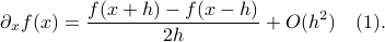
Now one might be tempted to make  extremely small, as then the error must vanish!
However, numerically, for a very small the two function evaluations
extremely small, as then the error must vanish!
However, numerically, for a very small the two function evaluations  and
and  will be indistinguishable.
So although the error scales as
will be indistinguishable.
So although the error scales as  there is some practical lower bound on this error based on the machine precision of your computer.
One potential application of numerical derivatives is in the context of zeroth-order (derivative-free) optimization.
Say you want to adjust van der Poel his Canyon frame such that he goes even faster, you will not have access to explicit gradients, but you can evaluate the performance of a change in design, for example in a simulator. So what you usually can obtain is a set of function evaluations
there is some practical lower bound on this error based on the machine precision of your computer.
One potential application of numerical derivatives is in the context of zeroth-order (derivative-free) optimization.
Say you want to adjust van der Poel his Canyon frame such that he goes even faster, you will not have access to explicit gradients, but you can evaluate the performance of a change in design, for example in a simulator. So what you usually can obtain is a set of function evaluations  . Given this data, a somewhat obvious approach is to mimick first-order algorithms

where  is some stepsize. For example, one could replace
  in by the central-difference approximation .
Clearly, if the objective function is well-behaved and the approximation of is reasonably good, then something must come out?
As was remarked before, if your approximation - for example due to numerical cancellation errors - will always have a bias it is not immediate how to construct a high-performance zeroth-order optimization algorithm. Only if there was a way to have a numerical approximation without finite differencing?
in by the central-difference approximation .
Clearly, if the objective function is well-behaved and the approximation of is reasonably good, then something must come out?
As was remarked before, if your approximation - for example due to numerical cancellation errors - will always have a bias it is not immediate how to construct a high-performance zeroth-order optimization algorithm. Only if there was a way to have a numerical approximation without finite differencing?
Let us assume that  is sufficiently smooth, let be the imaginary number and consider the following series

From this expression it follows that
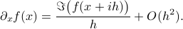
So we see that by passing to the complex domain and projecting the imaginary part back, we obtain a numerical method to construct approximations of derivatives without even the possibility of cancellation errors. This remarkable property makes it a very attractive candidate to be used in zeroth-order optimization algorithms, which is precisely what we investigated in our new pre-print. It turns out that convergence is not only robust, but also very fast!
Optimal coordinates |24 May 2020|
tags: math.LA, math.OC, math.DS
There was a bit of radio silence, but as indicated here, some interesting stuff is on its way.
In this post we highlight this 1976 paper by Mullis and Roberts on ’Synthesis of Minimum Roundoff Noise Fixed Point Digital Filters’.
Let us be given some single-input single-output (SISO) dynamical system 
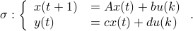
It is known that the input-output behaviour of any  , that is, the map from
  to is invariant under a similarity transform.
To be explicit, the tuples
to is invariant under a similarity transform.
To be explicit, the tuples  and
and  , which correspond to the change of coordinates
  for some
  , give rise to the same input-output behaviour.
Hence, one can define the equivalence relation
, give rise to the same input-output behaviour.
Hence, one can define the equivalence relation  by imposing that the input-output maps of and
  are equivalent.
By doing so we can consider the quotient
are equivalent.
By doing so we can consider the quotient  . However, in practice, given a , is any such that
  equally useful?
For example, the following and
equally useful?
For example, the following and  are similar, but clearly, is preferred from a numerical point of view:
![A = left[begin{array}{ll} 0.5 & 10^9 0 & 0.5 end{array}right],quad A' = left[begin{array}{ll} 0.5 & 1 0 & 0.5 end{array}right].](eqs/6214495422406291774-130.png)
In what follows, we highlight the approach from Mullis and Roberts and conclude by how to optimally select . Norms will be interpreted in the  sense, that is, for
  ,
,  . Also, in what follows we assume that
  plus that is stable, which will mean
  and that corresponds to a minimal realization.
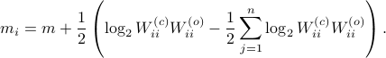
The first step is to quantify the error. Assume we have allocated  bits at our disposal to present the
  component of
  . These values for can differ, but we constrain the average by
  for some
  . Let
. Let  be a 'step-size’, such that our dynamic range of
  is bounded by
  (these are our possible representations). Next we use the modelling choices from Mullis and Roberts, of course, they are debatable, but still, we will infer some nice insights.
First, to bound the dynamic range, consider solely the effect of an input, that is, define  by
by  ,
,  . Then we will impose the bound
  on . In combination with the step size (quantization), this results in
  . Let
. Let  be a sequence of i.i.d. sampled random variables from
  . Then we see that
  . Hence, one can think of
  as scaling parameter related to the probability with which this dynamic range bound is true.
Next, assume that all the round-off errors are independent and have a variance of  .
Hence, the worst-case variance of computating
.
Hence, the worst-case variance of computating  is
is  . To evaluate the effect of this error on the output, assume for the moment that is identically
  .
Then,
.
Then, 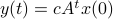 . Similar to , define
  as the component of
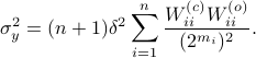
  . As before we can compute the variance, this time of the full output signal, which yields
 . Note, these expressions hinge on the indepedence assumption.
Next, define the (infamous) matrices  ,
,  by
by
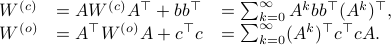
If we assume that the realization is not just minimal, but that  is a controllable pair and that
  is an observable pair, then,
  and
and  .
Now the key observation is that
.
Now the key observation is that 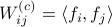 and similarly
 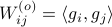 .
Hence, we can write
.
Hence, we can write 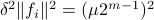 as
as  and indeed
  .
Using these Lyapunov equations we can say goodbye to the infinite-dimensional objects.
.
Using these Lyapunov equations we can say goodbye to the infinite-dimensional objects.
To combine these error terms, let say we have apply a coordinate transformation  , for some .
Specifically, let be diagonal and defined by
, for some .
Specifically, let be diagonal and defined by  .
Then one can find that
.
Then one can find that 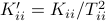 ,
,  . Where the latter expressions allows to express the output error (variance) by
Now we want to minimize  over all plus some optimal selection of . At this point it looks rather painful. To make it work we first reformulate the problem using the well-known arithmetic-geometric mean inequality
![^{[1]}](eqs/2708305882951756665-130.png) for non-negative sequences
for non-negative sequences ![{a_i}_{iin [n]}](eqs/351138265746961916-130.png) :
:
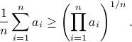
This inequality yields

See that the right term is independent of , hence this is a lower-bound with respect to minimization over . To achieve this (to make the inequality from an equality), we can select
Indeed, as remarked in the paper, is not per se an integer. Nevertheless, by this selection we find the clean expression from to minimize over systems equivalent to , that is, over some transformation matrix . Define a map ![f:mathcal{S}^n_{succ 0}to (0,1]](eqs/6462334851245421111-130.png) by
by
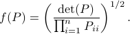
It turns out that  if and only if
  is diagonal. This follows
![^{[2]}](eqs/2708306882823756034-130.png) from Hadamard's inequality.
We can use this map to write
from Hadamard's inequality.
We can use this map to write

Since the term  is invariant under a transformation , we can only optimize over a structural change in realization tuple , that is, we need to make
  and
and  simultaneous diagonal! It turns out that this numerically 'optimal’ realization, denoted
  , is what is called a principal axis realization.
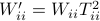
To compute it, diagonalize ,  and define
  . Next, construct the diagonalization
  . Then our desired transformation is
  . First, recall that under any the pair
  becomes
  . Plugging in our map yields the transformed matrices
  , which are indeed diagonal.
 |
At last, we do a numerical test in Julia. Consider a linear system ![A = left[begin{array}{ll} 0.8 & 0.001 0 & -0.5 end{array} right],quad b = left[begin{array}{l} 10 0.1 end{array} right],](eqs/3623138148766993767-130.png)
![c=left[begin{array}{ll} 10 & 0.1 end{array} right],quad d=0.](eqs/42331078943303768-130.png)
To simulate numerical problems, we round the maps |
 and
and  to the closest integer where
 ![[cdot]](eqs/8251583936328055799-130.png) , naive realization
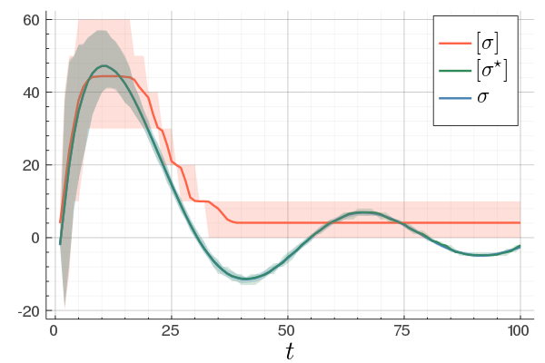
, naive realization ![[sigma]](eqs/4713363484184404481-130.png) and to the optimized one
and to the optimized one ![[sigma^{star}]](eqs/5091401033446485837-130.png) .
We do 100 experiments and show the mean plus the full confidence interval (of the input-output behaviour), the optimized representation is remarkably better.
Numerically we observe that for
.
We do 100 experiments and show the mean plus the full confidence interval (of the input-output behaviour), the optimized representation is remarkably better.
Numerically we observe that for  , which is precisely where the naive
 ![[1]](eqs/8209412804330245758-130.png) : To show this AM-GM inequality, we can use Jensen's inequality for concave functions, that is,
: To show this AM-GM inequality, we can use Jensen's inequality for concave functions, that is, ![mathbf{E}[g(x)]leq g(mathbf{E}[x])](eqs/8492979742681909343-130.png) . We can use the logarithm as our prototypical concave function on
. We can use the logarithm as our prototypical concave function on  and find
  . Then, the result follows.
![[2]](eqs/8209412804333245623-130.png) : The inequality attributed to Hadamard is slightly more difficult to show. In its general form the statement is that
: The inequality attributed to Hadamard is slightly more difficult to show. In its general form the statement is that  , for
, for  the column of . The inequality becomes an equality when the columns are mutually orthogonal. The intuition is clear if one interprets the determinant as the signed volume spanned by the columns of , which. In case
  , we know that there is
  such that
  , hence, by this simple observation it follows that
Equality holds when the columns are orthogonal, so  must be diagonal, but
  must also hold, hence,
  must be diagonal, and thus must be diagonal, which is the result we use.
Risky Business in Stochastic Control: Exponential Utility |12 Jan. 2020|
tags: math.OC
One of the most famous problems in linear control theory is that of designing a control law which minimizes some cost being quadratic in input and state. We all know this as the Linear Quadratic Regulator (LQR) problem.
There is however one problem (some would call it a blessing) with this formulation once the dynamics contain some zero-mean noise: the control law is independent of this stochasticity. This is easy in proofs, easy in practice, but does it work well? Say, your control law is rather slow, but bringing you back to in the end of time. In the noiseless case, no problem. But now say there is a substantial amount of noise, do you still want such a slow control law? The answer is most likely no since you quickly drift away. The classical LQR formulation does not differentiate between noise intensities and hence can be rightfully called naive as Bertsekas did (Bert76). Unfortunately, this name did not stuck.
Can we do better? Yes. Define the cost function
![gamma_{T-1}(theta) = frac{2}{theta T}log mathbf{E}_{xi}left[mathrm{exp}left(frac{theta}{2}sum^{T-1}_{t=0}x_t^{top}Qx_t + u_t^{top}Ru_t right) right]=frac{2}{theta T}log mathbf{E}_{xi}left[mathrm{exp}left(frac{theta}{2}Psi right) right]](eqs/6416747510437753707-130.png)
and consider the problem of finding the minimizing policy  in:
in:

Which is precisely the classical LQR problem, but now with the cost wrapped in an exponential utility function parametrized by  .
This problem was pioneered by most notably Peter Whittle (Wh90).
.
This problem was pioneered by most notably Peter Whittle (Wh90).
Before we consider solving this problem, let us interpret the risk parameter . For  we speak of a risk-sensitive formulation while for
  we are risk-seeking. This becomes especially clear when you solve the problem, but a quick way to see this is to consider the approximation of
  near
near  , which yields
 ![gammaapprox mathbf{E}[Psi]+frac{1}{4}{theta}mathbf{E}[Psi]^2](eqs/7712769251826009795-130.png) , so
, so  relates to pessimism and to optimism indeed. Here we skipped a few scaling factors, but the idea remains the same, for a derivation, consider cumulant generating functions and have a look at our problem.
As with standard LQR, we would like to obtain a stabilizing policy and to that end we will be mostly bothered with solving  .
However, instead of immediately trying to solve the infinite horizon average cost Bellman equation it is easier to consider
.
However, instead of immediately trying to solve the infinite horizon average cost Bellman equation it is easier to consider  for finite first. Then, when we can prove monotonicty and upper-bound
  , the infinite horizon optimal policy is given by
  .
The reason being that monotonic sequences which are uniformly bounded converge.
.
The reason being that monotonic sequences which are uniformly bounded converge.
The main technical tool towards finding the optimal policy is the following Lemma similar to one in the Appendix of (Jac73):
Lemma 
Consider a noisy linear dynamical system defined by  with
with 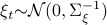 and let
  be shorthand notation for
  . Then, if
  holds we have
![mathbf{E}_{xi}left[mathrm{exp}left(frac{theta}{2}x_{k+1}^{top}Px_{k+1} right)|x_kright] = frac{|(Sigma_{xi}-theta D^{top}PD)^{-1}|^{1/2}}{|Sigma_{xi}^{-1}|^{1/2}}mathrm{exp}left(frac{theta}{2}(Ax_k+Bu_k)^{top}widetilde{P}(Ax_k+Bu_k) right)](eqs/8871996922177725349-130.png)
where
 .
. 
Proof
Let ![z:= mathbf{E}_{xi}left[mathrm{exp}left(frac{theta}{2}x_{t+1}^{top}Px_{t+1} right)|x_tright]](eqs/2205886115745182034-130.png) and recall that the shorthand notation for is , then:
and recall that the shorthand notation for is , then:
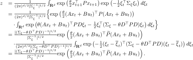
Here, the first step follows directly from  being a zero-mean Gaussian. In the second step we plug in
  . Then, in the third step we introduce a variable
  with the goal of making
  the covariance matrix of a Gaussian with mean . We can make this work for

and additionally

Using this approach we can integrate the latter part to  and end up with the final expression.
Note that in this case the random variable
and end up with the final expression.
Note that in this case the random variable  needs to be Gaussian, since the second to last expression in
  equals by being a Gaussian probability distribution integrated over its entire domain.
What is the point of doing this?
Let 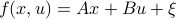 and assume that
 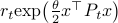 represents the cost-to-go from stage
  and state . Then consider
![r_{t-1}mathrm{exp}left(frac{theta}{2}x^{top}P_{t-1} xright) = inf_{u} left{mathrm{exp}left(frac{theta}{2}(x^{top}Qx+u^{top}Ru)right)mathbf{E}_{xi}left[r_tmathrm{exp}left( frac{theta}{2}f(x,u)^{top}P_{t}f(x,u)right);|;xright]right}.](eqs/8431854396343916570-130.png)
Note, since we work with a sum within the exponent, we must multiply within the right-hand-side of the Bellman equation.
From there it follows that
 , for
, for


The key trick in simplifying your expressions is to apply the logarithm after minimizing over such that the fraction of determinants becomes a state-independent affine term in the cost.
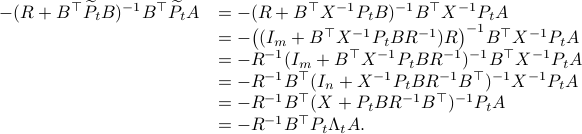
Now, using a matrix inversion lemma and the push-through rule we can remove  and construct a map
  :
:

such that 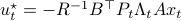 .
See below for the derivations, many (if not all) texts skip them, but if you have never applied the push-through rule they are not that obvious.
.
See below for the derivations, many (if not all) texts skip them, but if you have never applied the push-through rule they are not that obvious.
As was pointed out for the first time by Jacobson (Jac73), these equations are precisely the ones we see in (non-cooperative) Dynamic Game theory for isotropic  and appropriately scaled
  .
.
Especially with this observation in mind there are many texts which show that  is well-defined and finite, which relates to finite cost and a stabilizing control law
  . To formalize this, one needs to assume that
  is a minimal realization for defined by
  . Then you can appeal to texts like (BB95).
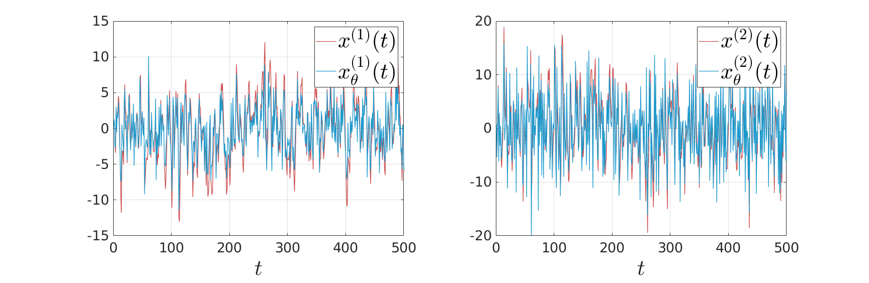
Numerical Experiment and Robustness Interpretation
To show what happens, we do a small -dimensional example. Here we want to solve the Risk-Sensitive  ) and the Risk-neutral () infinite-horizon average cost problem for
![A = left[ begin{array}{ll} 2 & 1 0 & 2 end{array}right],quad B = left[ begin{array}{l} 0 1 end{array}right],quad Sigma_{xi}^{-1} = left[ begin{array}{ll} 10^{-1} & 200^{-1} 200^{-1} & 10 end{array}right],](eqs/5026564260006708683-130.png)
 ,
,  ,
,  .
There is clearly a lot of noise, especially on the second signal, which also happens to be critical for controlling the first state. This makes it interesting.
We compute
.
There is clearly a lot of noise, especially on the second signal, which also happens to be critical for controlling the first state. This makes it interesting.
We compute  and
and  .
Given the noise statistics, it would be reasonable to not take the certainty equivalence control law
.
Given the noise statistics, it would be reasonable to not take the certainty equivalence control law  since you control the first state (which has little noise on its line) via the second state (which has a lot of noise on its line). Let
  be the state under and
  the state under
  .
.
We see in the plot below (for some arbitrary initial condition) typical behaviour, does take the noise into account and indeed we see the induces a smaller variance.
 |
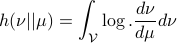
So, is more robust than in a particular way. It turns out that this can be neatly explained. To do so, we have to introduce the notion of Relative Entropy (Kullback-Leibler divergence). We will skip a few technical details (see the references for full details). Given a measure  on
on  , then for any other measure
  , being absolutely continuous with respect to (
 ), define the Relative Entropy as:
Now, for any measurable function  on , being bounded from below, it can be shown (see (DP96)) that
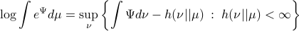
For the moment, think of as your standard finite-horizon LQR cost with product measure  , then we see that an exponential utility results in the understanding that a control law which minimizes
  is robust against adversarial noise generated by distributions sufficiently close (measured by ) to the reference .
Here we skipped over a lot of technical details, but the intuition is beautiful, just changing the utility to the exponential function gives a wealth of deep distributional results we just touched upon in this post.
Simplification steps in 
We only show to get the simpler representation for the input, the approach to obtain  is very similar.
First, using the matrix inversion lemma:

we rewrite into:

Note, we factored our  since we cannot assume that is invertible. Our next tool is called the push-through rule. Given
  and
and  we have

You can check that indeed  .
Now, to continue, plug this expression for into the input expression:
.
Now, to continue, plug this expression for into the input expression:
Indeed, we only used factorizations and the push-through rule to arrive here.
(Bert76) Dimitri P. Bertsekas : ‘‘Dynamic Programming and Stochastic Control’’, 1976 Academic Press.
(Jac73) D. Jacobson : ‘‘Optimal stochastic linear systems with exponential performance criteria and their relation to deterministic differential games’’, 1973 IEEE TAC.
(Wh90) Peter Whittle : ‘‘Risk-sensitive Optimal Control’’, 1990 Wiley.
(BB95) Tamer Basar and Pierre Bernhard : ‘‘-Optimal Control and Related Minimax Design Problems A Dynamic Game Approach’’ 1995 Birkhauser.
(DP96) Paolo Dai Pra, Lorenzo Meneghini and Wolfgang J. Runggaldier :‘‘Connections Between Stochastic Control and Dynamic Games’’ 1996 Math. Control Signals Systems.
Are Theo Jansen his Linkages Optimal? |16 Dec. 2019|
tags: math.OC, other.Mech
Theo Jansen, designer of the infamous ‘‘strandbeesten’’ explains in a relatively recent series of videos that the design of his linkage system is the result of what could be called an early implementation of genetic programming. Specifically, he wanted the profile that the foot follows to be flat on the bottom. He does not elaborate on this too much, but the idea is that in this way his creatures flow over the surface instead of the more bumpy motion we make. Moreover, you can imagine that in this way the center of mass remains more or less at a constant height, which is indeed energy efficient. Now, many papers have been written on understanding his structure, but I find most of them rather vague, so lets try a simple example.
To that end, consider just 1 leg, 1 linkage system as in the figure(s) below. We can write down an explicit expression for  where
where  and
and  . See below for an explicit derivation. Now, with his motivation in mind, what would be an easy and relevant cost function? An idea is to maximize the ratio
  , of course, subject to still having a functioning leg. To that end we consider the cost function (see the schematic below for notation):
Of course, this is a heuristic, but the intuition is that this should approximate .
Let  be the set of parameters as given in Jansen his video, then we apply a few steps of (warm-start) gradient ascent:
 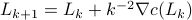 ,
,  .
.
 |
In the figure on the left we compare the linkage as given by Jansen (in black) with the result of just two steps of gradient ascent (in red).
You clearly see that the trajectory of the foot becomes more shallow. Nevertheless, we see that the profile starts to become curved on the bottom. It is actually interesting to note that |
 , which is still far from
  .
. Can we conclude anything from here? I would say that we need dynamics, not just kinematics, but more importantly, we need to put the application in the optimization and only Theo Jansen understands the constraints of the beach.
Still, it is fun to see for yourself how this works and like I did you can build a (baby) strandbeest yourself using nothing more than some PVC tubing and a source of heat.
Derivation of  :
:
Essentially, all that you need is the cosine-rule plus some feeling for how to make the equations continuous.
To start, let  and
and  (just the standard unit vectors), plus let
  be a standard (counter-clockwise) rotation matrix acting on
  . To explain the main approach, when we want to find the coordinates of for example point
  , we try to compute the angle
  such that when we rotate the unit vector
  with length
  emanating from point
  , we get point . See the schematic picture below.
Then we easily obtain  ,
,  and
and  .
Now, to obtain and
.
Now, to obtain and  compute the length of the diagonal,
  and using the cosine rule
  ,
,  . Then, the trick is to use
  to compute
  . To avoid angles larger than , consider an inner product with
  and add the remaining
  ;
;  . From there we get
  ,
,  ,
,  ,
,  . The point
  is not missing, to check your code it is convenient to compute
  and check that agrees with
  for all
  .
In a similar fashion,
.
In a similar fashion,  ,
,  ,
,  .
Then, for
.
Then, for  , again compute a diagonal
  plus
plus  ,
, 
 , such that for
 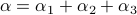 we have
  .
At last,
.
At last,  , such that
  for
for  .
.
 |