Co-observability |6 January 2022|
`tags: math.OC`

A while ago Prof. Jan H. van Schuppen published his book Control and System Theory of Discrete-Time Stochastic Systems. In this post I would like to highlight one particular concept from the book: (stochastic) co-observability, which is otherwise rarely discussed.

We start with recalling observability. Given a linear-time-invariant system with $xin mathbf{R}^n$ , $yin mathbf{R}^p$ :

$Sigma :left{ begin{array}{ll} x(t+1) &= Ax(t),quad x(0)=x_0 y(t) &= Cx(t) end{array}right.$

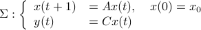
one might wonder if the initial state x_0 can be recovered from a sequence of outputs y(0),dots,y(k) . (This is of great use in feedback problems.) By observing that y(0)=Cx(0) , y(1)=CAx(0) , y(2)=CA^2x(0) one is drawn to the observability matrix

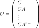
$mathcal{O}= left( begin{array}{l} C CA vdots CA^{n-1} end{array} right)$

Without going into detectability, when mathcal{O} is full-rank, one can (uniquely) recover x_0 (proof by contradiction). If this is the case, we say that Sigma , or equivalenty the pair (A,C) , is observable. Note that using a larger matrix (more data) is redudant by the Cayley-Hamilton theorem (If would not be full-rank, but by adding CA^n “from below” it would somehow be full-rank, one would contradict the Cayley-Hamilton theorem.). Also note that in practice one does not “invert” mathcal{O} but rather uses a (Luenberger) observer (or a Kalman filter).

Now lets continue with a stochastic (Gaussian) system, can we do something similar? Here it will be even more important to only think about observability matrices as merely tools to assert observability. Let $v:Omegatomathbf{R}^v$ be a zero-mean Gaussian random variable with covariance Q_v and define for some matrices and the stochastic system

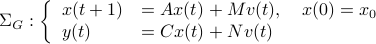
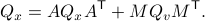
$Sigma_G :left{ begin{array}{ll} x(t+1) &= Ax(t)+Mv(t),quad x(0)=x_0 y(t) &= Cx(t)+Nv(t) end{array}right.$

We will assume that is asymptotically (exponentially stable) such that the Lyapunov equation describing the (invariant) state-covariance is defined:

$Q_x = AQ_xA^{mathsf{T}}+MQ_vM^{mathsf{T}}.$

Now the support of the state is the range of Q_x .

A convenient tool to analyze Sigma_G will be the characteristic function of a Gaussian random variable , defined as varphi(omega)=mathbf{E}[mathrm{exp}(ilangle omega, Xrangle)] . It can be shown that for a Gaussian random variable sim G(mu,Q) $varphi(omega)=mathrm{exp}(ilangle omega,murangle - frac{1}{2}langle omega, Qomega rangle)$ . With this notation fixed, we say that $Sigma_{G}$ is stochastically observable on the internal t,dots,t+k if the map

$x(t)mapsto mathbf{E}[mathrm{exp}(ilangle omega,bar{y}rangle|mathcal{F}^{x(t)}],quad bar{y}=(y(t),dots,y(t+k))in mathbf{R}^{pcdot(k+1)}quad forall omega$

is injective on the support of (note the forall omega ). The intuition is the same as before, but now we want the state to give rise to an unique (conditional) distribution. At this point is seems rather complicated, but as it turns out, the conditions will be similar to ones from before. We start by writing down explicit expressions for bar{y} , as

$y(t+s) = CA^s x(t) + sum^{t+s-1-i}_{i=0}CA^i M v(t+s-1-i) + N v(t+s)$

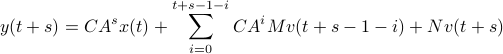
we find that

$bar{y} = mathcal{O}_k x(t) + mathcal{M}_k bar{v},$

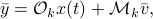
for $mathcal{O}_k$ the observability matrix corresponding to the data (length) of bar{y} , $mathcal{M}_k$ a matrix containing all the noise related terms and bar{v} a stacked vector of noises similar to bar{y} . It follows that $x(t)mapsto mathbf{E}[mathrm{exp}(ilangle omega,bar{y})|mathcal{F}^{x(t)}]$ is given by $mathrm{exp}(ilangle omega, mathcal{O}_k x(t)rangle - frac{1}{2}langle omega, mathcal{Q}_komega rangle)$ , for $mathcal{Q}_k = mathbf{E}[mathcal{M}_kbar{v}bar{v}^{mathsf{T}}mathcal{M}_k^{mathsf{T}}]$ . Injectivity of this map clearly relates directly to injectivity of $x(t)mapsto mathcal{O}_k x(t)$ . 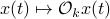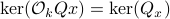As such (taking the support into account), a neat characterization of stochastic observability is that $mathrm{ker}(mathcal{O}_kQx)=mathrm{ker}(Q_x)$ .

Then, to introduce the notion of stochastic co-observability we need to introduce the backward representation of a system. We term system representations like Sigma and Sigma_G “forward” representations as tto +infty . Assume that Q_xsucc 0 , then see that the forward representation of a system matrix, denoted A^f is given by $A^f = mathbf{E}[x(t+1)x(t)^{mathsf{T}}]Q_x^{-1}$ . In a similar vein, the backward representation is given by $A^b=mathbf{E}[x(t-1)x(t)^{mathsf{T}}]Q_x^{-1}$ . Doing the same for the output matrix yields $C^b=mathbf{E}[y(t-1)x(t)^{mathsf{T}}]Q_x^{-1}$ and thereby the complete backward system

$Sigma^b_G :left{ begin{array}{ll} x(t-1) &= A^bx(t)+Mv(t),quad x(0)=x_0 y(t-1) &= C^bx(t)+Nv(t) end{array}right.$

Note, to keep and fixed, we adjust the distribution of . Indeed, when Q_x is not full-rank, the translation between forward and backward representations is not well-defined. Initial conditions $x_0in mathrm{ker}(Q_x)$ cannot be recovered.

To introduce co-observability, ignore the noise for the moment and observe that y(t-1)=C^bx(t) , y(t-2)=C^bA^bx(t) , and so forth. We see that when looking at observability using the backward representation, we can ask if it possible to recover the current state using past outputs. Standard observability looks at past states instead. With this in mind we can define stochastic co-observability on the interval t-k-1,dots,t-1 be demanding that the map

$x(t)mapsto mathbf{E}[mathrm{exp}(ilangle omega,bar{y}^brangle|mathcal{F}^{x(t)}],quad bar{y}^b=(y(t-1),dots,y(t-k-1))in mathbf{R}^{pcdot(k+1)}quad forall omega$

is injective on the support of (note the forall omega ). Of course, one needs to make sure that y(t-k-1) is defined. It is no surprise that the conditions for stochastic co-observability will also be similar, but now using the co-observability matrix. What is however remarkable, is that these notions do not always coincide.

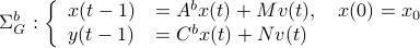
Lets look at when this can happen and what this implies. One reason to study these kind of questions is to say something about (minimal) realizations of stochastic processes. Simply put, what is the smallest (as measured by the dimension of the state ) system Sigma_G that gives rise to a certain output process. When observability and co-observability do not agree, this indicates that the representation is not minimal. To get some intuition, we can do an example as adapted from the book. Consider the scalar (forward) Gaussian system

$Sigma^f_G :left{ begin{array}{ll} x(t+1) &= ax(t)+mv(t),quad x(0)=x_0,quad ain (-1,1) setminus{0},quad m=(a^2-1)/a y(t) &= x(t)+v(t) end{array}right.$

for vsim G(0,1) . The system is stochastically observable as cneq 0 and q_x=(1-a)^2/a^2neq 0 . Now for stochastic co-observability we see that $c^b=mathbf{E}[y(t-1)x(t)]q_x^{-1}]=0$ , as such the system is not co-observable. What this shows is that y(t) behaves as a Gaussian random variable, no internal dynamics are at play and such a minimal realization is of dimension n=0 .

For this and a lot more, have a look at the book!

Co-observability |6 January 2022|tags: math.OC

Co-observability |6 January 2022|
`tags: math.OC`