Optimal coordinates |24 May 2020|
tags: math.LA, math.OC, math.DS
In this post we highlight this 1976 paper by Mullis and Roberts on ’Synthesis of Minimum Roundoff Noise Fixed Point Digital Filters’.
Let us be given some single-input single-output (SISO) dynamical system 
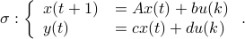
It is known that the input-output behaviour of any  , that is, the map from
  to
to  is invariant under a similarity transform.
To be explicit, the tuples
is invariant under a similarity transform.
To be explicit, the tuples  and
and 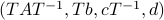 , which correspond to the change of coordinates
  for some
  , give rise to the same input-output behaviour.
Hence, one can define the equivalence relation
, give rise to the same input-output behaviour.
Hence, one can define the equivalence relation  by imposing that the input-output maps of and
  are equivalent.
By doing so we can consider the quotient
are equivalent.
By doing so we can consider the quotient  . However, in practice, given a , is any such that
  equally useful?
For example, the following
equally useful?
For example, the following  and
and  are similar, but clearly, is preferred from a numerical point of view:
![A = left[begin{array}{ll} 0.5 & 10^9 0 & 0.5 end{array}right],quad A' = left[begin{array}{ll} 0.5 & 1 0 & 0.5 end{array}right].](eqs/6214495422406291774-130.png)
In what follows, we highlight the approach from Mullis and Roberts and conclude by how to optimally select . Norms will be interpreted in the  sense, that is, for
  ,
, 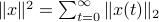 . Also, in what follows we assume that
  plus that is stable, which will mean
  and that corresponds to a minimal realization.
The first step is to quantify the error. Assume we have allocated  bits at our disposal to present the
  component of
  . These values for can differ, but we constrain the average by
 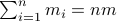 for some
  . Let
. Let  be a 'step-size’, such that our dynamic range of
  is bounded by
  (these are our possible representations). Next we use the modelling choices from Mullis and Roberts, of course, they are debatable, but still, we will infer some nice insights.
First, to bound the dynamic range, consider solely the effect of an input, that is, define  by
by  ,
,  . Then we will impose the bound
  on . In combination with the step size (quantization), this results in
  . Let
. Let  be a sequence of i.i.d. sampled random variables from
  . Then we see that
  . Hence, one can think of
  as scaling parameter related to the probability with which this dynamic range bound is true.
Next, assume that all the round-off errors are independent and have a variance of  .
Hence, the worst-case variance of computating
.
Hence, the worst-case variance of computating  is
is  . To evaluate the effect of this error on the output, assume for the moment that is identically
  .
Then,
.
Then, 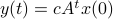 . Similar to , define
  as the component of
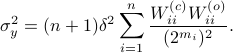
  . As before we can compute the variance, this time of the full output signal, which yields
 . Note, these expressions hinge on the indepedence assumption.
Next, define the (infamous) matrices  ,
,  by
by
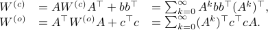
If we assume that the realization is not just minimal, but that  is a controllable pair and that
  is an observable pair, then,
  and
and  .
Now the key observation is that
.
Now the key observation is that 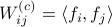 and similarly
 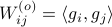 .
Hence, we can write
.
Hence, we can write  as
as  and indeed
  .
Using these Lyapunov equations we can say goodbye to the infinite-dimensional objects.
.
Using these Lyapunov equations we can say goodbye to the infinite-dimensional objects.
To combine these error terms, let say we have apply a coordinate transformation  , for some .
Specifically, let
, for some .
Specifically, let  be diagonal and defined by
  .
Then one can find that
.
Then one can find that  ,
,  . Where the latter expressions allows to express the output error (variance) by
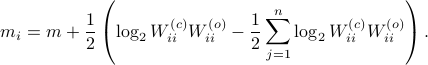
Now we want to minimize  over all plus some optimal selection of . At this point it looks rather painful. To make it work we first reformulate the problem using the well-known arithmetic-geometric mean inequality
![^{[1]}](eqs/2708305882951756665-130.png) for non-negative sequences
for non-negative sequences ![{a_i}_{iin [n]}](eqs/351138265746961916-130.png) :
:
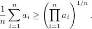
This inequality yields

See that the right term is independent of , hence this is a lower-bound with respect to minimization over . To achieve this (to make the inequality from  an equality), we can select
Indeed, as remarked in the paper, is not per se an integer. Nevertheless, by this selection we find the clean expression from to minimize over systems equivalent to , that is, over some transformation matrix . Define a map ![f:mathcal{S}^n_{succ 0}to (0,1]](eqs/6462334851245421111-130.png) by
by
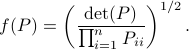
It turns out that  if and only if
  is diagonal. This follows
![^{[2]}](eqs/2708306882823756034-130.png) from Hadamard's inequality.
We can use this map to write
from Hadamard's inequality.
We can use this map to write

Since the term  is invariant under a transformation , we can only optimize over a structural change in realization tuple , that is, we need to make
  and
and  simultaneous diagonal! It turns out that this numerically 'optimal’ realization, denoted
  , is what is called a principal axis realization.
To compute it, diagonalize , 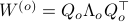 and define
  . Next, construct the diagonalization
  . Then our desired transformation is
  . First, recall that under any the pair
  becomes
  . Plugging in our map yields the transformed matrices
  , which are indeed diagonal.
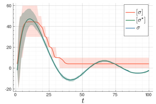 |
At last, we do a numerical test in Julia. Consider a linear system ![A = left[begin{array}{ll} 0.8 & 0.001 0 & -0.5 end{array} right],quad b = left[begin{array}{l} 10 0.1 end{array} right],](eqs/3623138148766993767-130.png)
![c=left[begin{array}{ll} 10 & 0.1 end{array} right],quad d=0.](eqs/42331078943303768-130.png)
To simulate numerical problems, we round the maps |
 and
and  to the closest integer where
 ![[cdot]](eqs/8251583936328055799-130.png) , naive realization
, naive realization ![[sigma]](eqs/4713363484184404481-130.png) and to the optimized one
and to the optimized one ![[sigma^{star}]](eqs/5091401033446485837-130.png) .
We do 100 experiments and show the mean plus the full confidence interval (of the input-output behaviour), the optimized representation is remarkably better.
Numerically we observe that for
.
We do 100 experiments and show the mean plus the full confidence interval (of the input-output behaviour), the optimized representation is remarkably better.
Numerically we observe that for  , which is precisely where the naive
 ![[1]](eqs/8209412804330245758-130.png) : To show this AM-GM inequality, we can use Jensen's inequality for concave functions, that is,
: To show this AM-GM inequality, we can use Jensen's inequality for concave functions, that is, ![mathbf{E}[g(x)]leq g(mathbf{E}[x])](eqs/8492979742681909343-130.png) . We can use the logarithm as our prototypical concave function on
. We can use the logarithm as our prototypical concave function on  and find
  . Then, the result follows.
![[2]](eqs/8209412804333245623-130.png) : The inequality attributed to Hadamard is slightly more difficult to show. In its general form the statement is that
: The inequality attributed to Hadamard is slightly more difficult to show. In its general form the statement is that 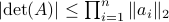 , for
, for  the column of . The inequality becomes an equality when the columns are mutually orthogonal. The intuition is clear if one interprets the determinant as the signed volume spanned by the columns of , which. In case
  , we know that there is
  such that
  , hence, by this simple observation it follows that
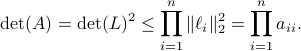
Equality holds when the columns are orthogonal, so  must be diagonal, but
  must also hold, hence,
  must be diagonal, and thus must be diagonal, which is the result we use.