Posts (2) containing the 'math.DG’ (Differential Geometry) tag:
Solving Linear Programs via Isospectral flows |05 September 2021|
tags: math.OC, math.DS, math.DG
In this post we will look at one of the many remarkable findings by Roger W. Brockett. Consider a Linear Program (LP)

parametrized by the compact set  and a suitable triple
  .
As a solution to
.
As a solution to  can always be found to be a vertex of
  , a smooth method to solve seems somewhat awkward.
We will see that one can construct a so-called isospectral flow that does the job.
Here we will follow Dynamical systems that sort lists, diagonalize matrices and solve linear programming problems, by Roger. W. Brockett (CDC 1988) and the book Optimization and Dynamical Systems edited by Uwe Helmke and John B. Moore (Springer 2ed. 1996).
Let have
, a smooth method to solve seems somewhat awkward.
We will see that one can construct a so-called isospectral flow that does the job.
Here we will follow Dynamical systems that sort lists, diagonalize matrices and solve linear programming problems, by Roger. W. Brockett (CDC 1988) and the book Optimization and Dynamical Systems edited by Uwe Helmke and John B. Moore (Springer 2ed. 1996).
Let have  vertices, then one can always find a map
  , mapping the simplex
  onto .
Indeed, with some abuse of notation, let
onto .
Indeed, with some abuse of notation, let  be a matrix defined as
  , for
, for  , the vertices of .
Before we continue, we need to establish some differential geometric results. Given the Special Orthogonal group  , the tangent space is given by
  . Note, this is the explicit formulation, which is indeed equivalent to shifting the corresponding Lie Algebra.
The easiest way to compute this is to look at the kernel of the map defining the underlying manifold.
. Note, this is the explicit formulation, which is indeed equivalent to shifting the corresponding Lie Algebra.
The easiest way to compute this is to look at the kernel of the map defining the underlying manifold.
Now, following Brockett, consider the function  defined by
  for some
  . This approach is not needed for the full construction, but it allows for more intuition and more computations.
To construct the corresponding gradient flow, recall that the (Riemannian) gradient at
. This approach is not needed for the full construction, but it allows for more intuition and more computations.
To construct the corresponding gradient flow, recall that the (Riemannian) gradient at  is defined via
 ![df(Theta)[V]=langle mathrm{grad},f(Theta), Vrangle_{Theta}](eqs/666734593389601294-130.png) for all
for all  . Using the explicit tangent space representation, we know that
  with
with  .
Then, see that by using
.
Then, see that by using

we obtain the gradient via
![df(Theta)[V]=lim_{tdownarrow 0}frac{f(Theta+tV)-f(Theta)}{t} = langle QTheta N, Theta Omega rangle - langle Theta N Theta^{mathsf{T}} Q Theta, Theta Omega rangle.](eqs/2651725126600601485-130.png)
This means that (the minus is missing in the paper) the (a) gradient flow becomes

Consider the standard commutator bracket ![[A,B]=AB-BA](eqs/2726051070798907854-130.png) and see that for
and see that for 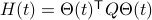 one obtains from the equation above (typo in the paper)
![dot{H}(t) = [H(t),[H(t),N]],quad H(0)=Theta^{mathsf{T}}QThetaquad (2).](eqs/8308117426617579905-130.png)
Hence,  can be seen as a reparametrization of a gradient flow.
It turns out that has a variety of remarkable properties. First of all, see that
can be seen as a reparametrization of a gradient flow.
It turns out that has a variety of remarkable properties. First of all, see that  preserves the eigenvalues of
  .
Also, observe the relation between extremizing
.
Also, observe the relation between extremizing  and the function
  defined via
  . The idea to handle LPs is now that the limiting will relate to putting weight one the correct vertex to get the optimizer,
  gives you this weight as it will contain the corresponding largest costs.
In fact, the matrix  can be seen as an element of the set
  .
This set is in fact a
.
This set is in fact a  -smooth compact manifold as it can be written as the orbit space corresponding to the group action
 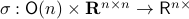 ,
,
 , one can check that this map satisfies the group properties. Hence, to extremize over
  , it appears to be appealing to look at Riemannian optimization tools indeed. When doing so, it is convenient to understand the tangent space of
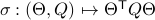
  . Consider the map defining the manifold
 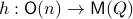 ,
,  . Then by the construction of
  , see that
 ![dh(Theta)[V]=0](eqs/8898228761859333701-130.png) yields the relation
yields the relation ![[H,Omega]=0](eqs/197549272010137556-130.png) for any
for any  .
.
For the moment, let  such that
  and
and  .
First we consider the convergence of .
Let have only distinct eigenvalues, then
.
First we consider the convergence of .
Let have only distinct eigenvalues, then  exists and is diagonal.
Using the objective from before, consider
exists and is diagonal.
Using the objective from before, consider  and see that by using the skew-symmetry one recovers the following
![begin{array}{lll} frac{d}{dt}mathrm{Tr}(H(t)N) &=& mathrm{Tr}(N [H,[H,N]]) &=& -mathrm{Tr}((HN-NH)^2) &=& |HN-NH|_F^2. end{array}](eqs/6018522323896655448-130.png)
This means the cost monotonically increases, but by compactness converges to some point  . By construction, this point must satisfy
 ![[H_{infty},N]=0](eqs/5408610946697229240-130.png) . As has distinct eigenvalues, this can only be true if itself is diagonal (due to the distinct eigenvalues).
. As has distinct eigenvalues, this can only be true if itself is diagonal (due to the distinct eigenvalues).
More can be said about , let  be the eigenvalues of
  , that is, they correspond to the eigenvalues of as defined above.
Then as preserves the eigenvalues of (), we must have
, that is, they correspond to the eigenvalues of as defined above.
Then as preserves the eigenvalues of (), we must have  , for
, for  a permutation matrix.
This is also tells us there is just a finite number of equilibrium points (finite number of permutations). We will write this sometimes as
a permutation matrix.
This is also tells us there is just a finite number of equilibrium points (finite number of permutations). We will write this sometimes as  .
.
Now as is one of those points, when does converge to ? To start this investigation, we look at the linearization of , which at an equilibrium point becomes

for  . As we work with matrix-valued vector fields, this might seems like a duanting computation. However, at equilibrium points one does not need a connection and can again use the directional derivative approach, in combination with the construction of
  , to figure out the linearization. The beauty is that from there one can see that is the only asymptotically stable equilibrium point of . Differently put, almost all initial conditions
  will converge to with the rate captured by spectral gaps in and . If does not have distinct eigenvalues and we do not impose any eigenvalue ordering on , one sees that an asymptotically stable equilibrium point must have the same eigenvalue ordering as . This is the sorting property of the isospectral flow and this is of use for the next and final statement.
Theorem:
Consider the LP with  for all
 ![i,jin [k]](eqs/5752860898065984697-130.png) , then, there exist diagonal matrices and
such that converges for almost any to
, then, there exist diagonal matrices and
such that converges for almost any to  with the optimizer of being
  .
.
Proof:
Global convergence is prohibited by the topology of .
Let  and let
  . Then, the isospectral flow will converge from almost everywhere to
  (only
(only  ), such that
  .
.
Please consider the references for more on the fascinating structure of .
Riemannian Gradient Flow |5 Nov. 2019|
tags: math.DG, math.DS
Previously we looked at  ,
,  - and its resulting flow - as the result from mapping
  to the sphere. However, we saw that for
  this flow convergences to
  , with
  such that for
  we have
 . Hence, it is interesting to look at the flow from an optimization point of view:
  .
.
A fair question would be, is our flow not simply Riemannian gradient ascent for this problem? As common with these kind of problems, such a hypothesis is something you just feel.
Now, using the tools from (CU1994, p.311) we can compute the gradient of  (on the sphere) via
  , where
  is a vector field normal to
  , e.g.,
  .
From there we obtain
.
From there we obtain
![mathrm{grad}_{mathbf{S}^2}(g|_{mathbf{S}^2}) = left[ begin{array}{lll} (1-x^2) & -xy & -xz -xy & (1-y^2) & -yz -xz & -yz & (1-z^2) end{array}right] left[ begin{array}{l}partial_x g partial_y g partial_z g end{array}right]=G(x,y,z)nabla g.](eqs/2499009703266316151-130.png)
To make our life a bit easier, use instead of the map  . Moreover, set
  . Then it follows that
![begin{array}{ll} mathrm{grad}_{mathbf{S}^2}(h|_{mathbf{S}^2}) &= left(I_3-mathrm{diag}(s)left[begin{array}{l} s^{top}s^{top}s^{top} end{array}right]right) 2A^{top}As &= 2left(A^{top}A-(s^{top}A^{top}Asright)I_3)s. end{array}](eqs/2245781100057659571-130.png)
Of course, to make the computation cleaner, we changed to  , but the relation between
  and is beautiful. Somehow, mapping trajectories of , for some , to the sphere corresponds to (Riemannian) gradient ascent applied to the problem
  .
.
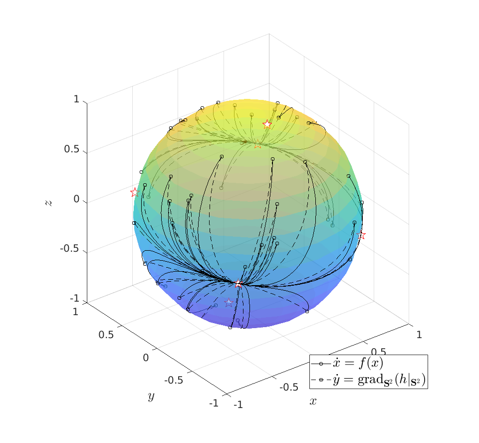 |
To do an example, let ![A = left[ begin{array}{lll} 10 & 2 & 0 2 & 10 & 2 0 & 2 & 1 end{array}right].](eqs/6133576945654762450-130.png)
We can compare |
 be given by
  . We see that the gradient flow under the quadratic function takes a clearly ‘‘shorter’’ path.
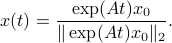
 Now, we formalize the previous analysis a bit a show how fast we convergence. Assume that the eigenvectors are ordered such that eigenvector  corresponds to the largest eigenvalue of . Then, the solution to
 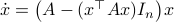 is given by
Let  be
be  expressed in eigenvector coordinates, with all
  (normalized). Moreover, assume all eigenvalues are distinct. Then, to measure if
  is near , we compute
  , which is
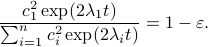
  if and only if is parallel to . To simplify the analysis a bit, we look at
 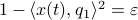 , for some perturbation
  , this yields
Next, take the the (natural) logarithm on both sides:
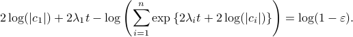
This log-sum-exp terms are hard to deal with, but we can apply the so-called ‘‘log-sum-exp trick’’:

In our case, we set 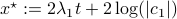 and obtain
![-log left(sum^{n}_{i=1}exp left{2 left[(lambda_i-lambda_1)t + logleft(frac{|c_i|}{|c_1|} right) right] right}+1 right) = log(1-varepsilon).](eqs/3165375830294523712-130.png)
We clearly observe that for  the LHS approaches from below, which means that
  from above, like intended. Of course, we also observe that the mentioned method is not completely general, we already assume distinct eigenvalues, but there is more. We do also not convergence when
  , which is however a set of measure on the sphere
  .
.
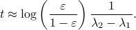
More interestingly, we see that the convergence rate is largely dictated by the ‘‘spectral gap/eigengap’’  . Specifically, to have a particular projection error
  , such that
  , we need
Comparing this to the resulting flow from  ,
,  , we see that we have the same flow, but with
  .
This is interesting, since
.
This is interesting, since  and
and  have the same eigenvectors, yet a different (scaled) spectrum. With respect to the convergence rate, we have to compare
  and
and  for any
  with
with  (the additional
  is not so interesting).
It is obvious what we will happen, the crux is, is  larger or smaller than
  ? Can we immediately extend this to a Newton-type algorithm? Well, this fails (globally) since we work in
  instead of purely with . To be concrete,
  , we never have
  degrees of freedom.
Of course, these observations turned out to be far from new, see for example (AMS2008, sec. 4.6).
(AMS2008) P.A. Absil, R. Mahony and R. Sepulchre: ‘‘Optimization Algorithms on Matrix Manifolds’’, 2008 Princeton University Press.
(CU1994) Constantin Udriste: ‘‘Convex Functions and Optimization Methods on Riemannian Manifolds’’, 1994 Kluwer Academic Publishers.