Riemannian Gradient Flow |5 Nov. 2019|
tags: math.DG, math.DS
Previously we looked at  ,
,  - and its resulting flow - as the result from mapping
  to the sphere. However, we saw that for
  this flow convergences to
  , with
  such that for
  we have
 . Hence, it is interesting to look at the flow from an optimization point of view:
  .
.
A fair question would be, is our flow not simply Riemannian gradient ascent for this problem? As common with these kind of problems, such a hypothesis is something you just feel.
Now, using the tools from (CU1994, p.311) we can compute the gradient of  (on the sphere) via
  , where
  is a vector field normal to
  , e.g.,
  .
From there we obtain
.
From there we obtain
![mathrm{grad}_{mathbf{S}^2}(g|_{mathbf{S}^2}) = left[ begin{array}{lll} (1-x^2) & -xy & -xz -xy & (1-y^2) & -yz -xz & -yz & (1-z^2) end{array}right] left[ begin{array}{l}partial_x g partial_y g partial_z g end{array}right]=G(x,y,z)nabla g.](eqs/2499009703266316151-130.png)
To make our life a bit easier, use instead of  the map
  . Moreover, set
  . Then it follows that
![begin{array}{ll} mathrm{grad}_{mathbf{S}^2}(h|_{mathbf{S}^2}) &= left(I_3-mathrm{diag}(s)left[begin{array}{l} s^{top}s^{top}s^{top} end{array}right]right) 2A^{top}As &= 2left(A^{top}A-(s^{top}A^{top}Asright)I_3)s. end{array}](eqs/2245781100057659571-130.png)
Of course, to make the computation cleaner, we changed to  , but the relation between
  and
and  is beautiful. Somehow, mapping trajectories of , for some , to the sphere corresponds to (Riemannian) gradient ascent applied to the problem
  .
.
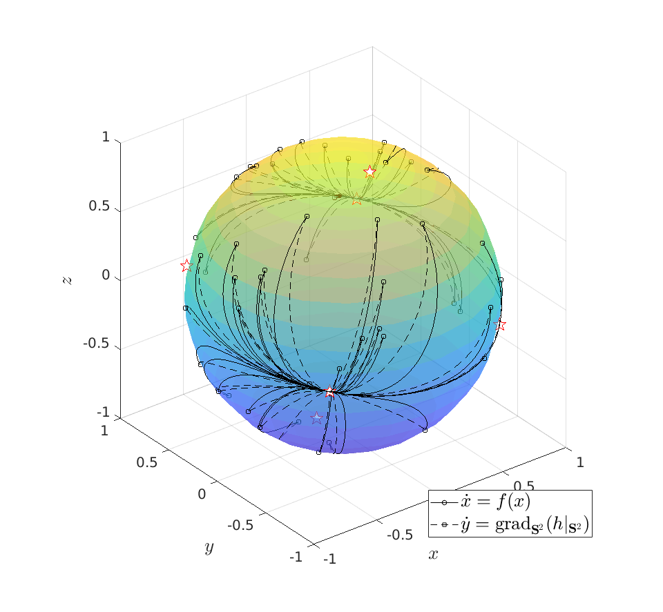 |
To do an example, let ![A = left[ begin{array}{lll} 10 & 2 & 0 2 & 10 & 2 0 & 2 & 1 end{array}right].](eqs/6133576945654762450-130.png)
We can compare |
 be given by
 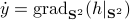 . We see that the gradient flow under the quadratic function takes a clearly ‘‘shorter’’ path.
 Now, we formalize the previous analysis a bit and show how fast we converge. Assume that the eigenvectors are ordered such that eigenvector  corresponds to the largest eigenvalue of . Then, the solution to
 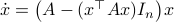 is given by
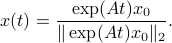
Let 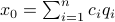 be
be  expressed in eigenvector coordinates, with all
  (normalized). Moreover, assume all eigenvalues are distinct. Then, to measure if
  is near , we compute
 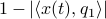 , which is
  if and only if is parallel to . To simplify the analysis a bit, we look at
 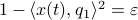 , for some perturbation
  , this yields
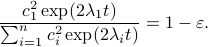
Next, take the the (natural) logarithm on both sides:
This log-sum-exp terms are hard to deal with, but we can apply the so-called ‘‘log-sum-exp trick’’:

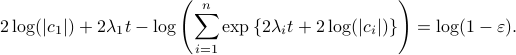
In our case, we set 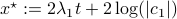 and obtain
![-log left(sum^{n}_{i=1}exp left{2 left[(lambda_i-lambda_1)t + logleft(frac{|c_i|}{|c_1|} right) right] right}+1 right) = log(1-varepsilon).](eqs/3165375830294523712-130.png)
We clearly observe that for  the LHS approaches from below, which means that
  from above, like intended. Of course, we also observe that the mentioned method is not completely general, we already assume distinct eigenvalues, but there is more. We do also not convergence when
  , which is however a set of measure on the sphere
  .
.
More interestingly, we see that the convergence rate is largely dictated by the ‘‘spectral gap/eigengap’’  . Specifically, to have a particular projection error
  , such that
  , we need
Comparing this to the resulting flow from  ,
,  , we see that we have the same flow, but with
  .
This is interesting, since
.
This is interesting, since  and
and  have the same eigenvectors, yet a different (scaled) spectrum. With respect to the convergence rate, we have to compare
  and
and  for any
  with
with  (the additional
  is not so interesting).
It is obvious what we will happen, the crux is, is  larger or smaller than
  ? Can we immediately extend this to a Newton-type algorithm? Well, this fails (globally) since we work in
  instead of purely with . To be concrete,
  , we never have
  degrees of freedom.
Of course, these observations turned out to be far from new, see for example (AMS2008, sec. 4.6).
(AMS2008) P.A. Absil, R. Mahony and R. Sepulchre: ‘‘Optimization Algorithms on Matrix Manifolds’’, 2008 Princeton University Press.
(CU1994) Constantin Udriste: ‘‘Convex Functions and Optimization Methods on Riemannian Manifolds’’, 1994 Kluwer Academic Publishers.