Recent news.
July 2026: Paper accepted for CDC26, see you between the waves!
July 2026: Poster presentation at BioControl26 in Oxford, see you in September!
July 2026: 2 talks at ECC26 (one regarding p53 at the "Robustness, resilience, and early warnings in natural dynamical networks" workshop and one during the regular track on a generalization of the Hartman-Grobman theorem).
June 2026: Pitch on "Necessary conditions for feedback stabilization of nontrivial attractors" at the Feedback Control of Biomedical Systems workshop at Digital Futures.
May 2026: Talk in the SysCon Seminar Series of Emering Academics at Uppsala University.
May 2026: Presentation at the Digital Futures Open Research Day 2026.
April 2026: 2 papers accepted for
IFAC WC 2026, see you in Korea!
March 2026: Abstract/poster accepted to the
p53 workshop, see you in Canada!
March 2026: Paper accepted for
ECC26, see you in Iceland!
March 2026: We have started posting
explanatory texts for the NCCR Automation. Short blogpost below.
March 2026: We organized the
DFYSC26. Short blogpost below.